前言
figures.zip · LiangCha_Xyy/Source – Gitee.com
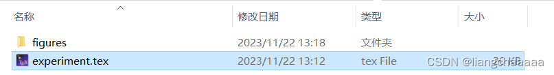
如下图,.tex文件和figures文件夹放在同一路径下即可

.tex代码
documentclass[UTF8]{ctexart}
usepackage{listings}
usepackage{xcolor}
usepackage{booktabs} %绘制表格
usepackage{caption2} %标题居中
usepackage{geometry}
usepackage{amsmath}
usepackage{amsfonts}
usepackage{amssymb}
usepackage{subfigure}
usepackage{longtable}
usepackage{float}
usepackage{graphicx}
usepackage{booktabs}
usepackage{indentfirst}
usepackage{setspace}
usepackage{adjustbox}

graphicspath{{figures/}}
geometry{a4paper,left=2.5cm,right=2.5cm,top=2.5cm,bottom=2.5cm}
setlength{parindent}{0em}
lstset{
	numbers=left, %设置行号位置
	numberstyle=tiny, %设置行号大小
	keywordstyle=color{blue}, %设置关键字颜色
	commentstyle=color[cmyk]{1,0,1,0}, %设置注释颜色
	escapeinside=``, %逃逸字符(1左面的键),用于显示中文
	%breaklines, %自动折行
	extendedchars=false, %解决代码跨页时,章节标题,页眉等汉字不显示的问题
	xleftmargin=1em,xrightmargin=1em, aboveskip=1em, %设置边距
	tabsize=4, %设置tab空格数
	showspaces=false %不显示空格
}
title{	}
author{自己的名字}
renewcommand{thesubsection}{thesection.arabic{subsection}}

begin{document}

begin{titlepage}
	centering
	vspace*{4cm} % 调整标题与图片的垂直间距
	includegraphics[scale=0.08]{logo.png} \
	{Huge Beijing University of Chemical Technology\} % 使用 Huge 调整字体大小
	{Huge Computing Methods\ }

	rule{15cm}{1.2pt}
	{Hugebfseries 计算方法课程实验\}
	rule{15cm}{1.2pt} \[2cm] % 调整标题与作者信息之间的垂直间距

	{Large 名字\[1cm]} % 调整作者信息的垂直间距
	{Large 日期\}
end{titlepage}
%实验二
section{Lagrange插值方法}
	subsection{实验目的}
		(1)熟悉简单的一阶和二阶 Lagrange插值方法;\
		(2)学会计算 Lagrange基函数;\
		(3)正确构造插值多项式;\
		(4)对插值结果进行合理分析;\

	subsection{实验原理}
		$p_n(x)=sum_{k=0}^n y_k l_k(x)=sum_{k=0}^nleft(prod_{substack{j=0 \ j neq k}}^n frac{x-x_j}{x_k-x_j}right) y_k$ \

	subsection{实验环境}
		Windows 10 + Visual Studio\

	subsection{实验内容}
		setstretch{1.5}
		centering
		begin{tabular}{|l|l|}
			hline$x$ & $f(x)$ \
			hline 24 & 1.888175 \
			26 & 1.918645 \
			28 & 1.947294 \
			30 & 1.961009 \
			hline
		end{tabular} \

		表 1.1: 数据样本表\
		vspace{0.5cm} % 插入垂直空白
		使用 Lagrange插值多项式计算 f(25),f(27),f(29),并给出插值多项式。\
		修改程序直至运行成功,查看运行结果,并和如下真实值进行比较。\
		vspace{0.5cm} % 插入垂直空白
		begin{tabular}{|l|l|}
			hline$x$ & $f(x)$ \
			hline
			25 & 1.90365393871587 \
			27 & 1.933182044931763 \
			29 & 1.961009057454548 \
			hline
		end{tabular} \
		表 1.2: 数据真实值\
		raggedright %左对齐
		vspace{5cm}
	subsection{程序代码}
		begin{lstlisting}[language=C++,basicstyle=small]
#include<iostream>
#include<cmath>
using namespace std;
int main()
{
	//输入程序
	int m;
	cout<<"请输入有几个采样点:"<<endl;
	cin>>m;
	pair<double,double> points[m];
	for(int i=0;i<m;i++){
		double x,y;
		cout<<"插值点:";
		cin>>x>>y;
		points[i] = {x,y};
		cout<<endl;
	}
	//程序处理
	int n;
	cout<<"请输入待预测的点的个数:"<<endl;
	cin>>n;
	for(int i=0;i<n;i++){
		double x_pred;
		cin>>x_pred;
		double res = 0;
		for(int j=0;j<m;j++){ // 使用 m 而不是 n
			double a = 1, b = 1;
			for(int k=0;k<m;k++){ // 修改内层循环变量名为 k
				if(j!=k){
					a *= (x_pred - points[k].first);
					b *= (points[j].first - points[k].first);
				}
			}
			res += a * points[j].second / b;
		}
		cout<<"插值点:(x,y)=("<<x_pred<<","<<res<<")"<<endl;
	}
}
		end{lstlisting}
		vspace{5cm}
		运行结果如下:\
		includegraphics[scale=0.8]{output1.png} \

%实验二
section{牛顿插值方法}
	subsection{实验目的}
	(1)理解牛顿插值方法;\
	(2)学会计算差商;\
	(3)正确构造插值多项式;\
	(4)设计程序并调试得到正确结果;

	subsection{实验原理}
	$fleft(x_0, x_1, cdots, x_nright)=sum_{k=0}^n frac{fleft(x_kright)}{prod_{substack{j=0 \ j neq k}}^nleft(x_k-x_jright)}$ \
	$n$ 次插值多项式:\
	$
	begin{aligned}
		p_{n}(x) & =fleft(x_0right)+fleft(x_0, x_1right)left(x-x_0right)+fleft(x_0, x_1, x_2right)left(x-x_0right)left(x-x_1right)+cdots \
		& +fleft(x_0, x_1, cdots, x_nright)left(x-x_0right)left(x-x_1right) cdotsleft(x-x_{n-1}right)
	end{aligned}
	$
	subsection{实验环境}
	Windows 10 + Visual Studio
	subsection{实验内容}
	计算以下积分值:\
	setstretch{1.5}
	centering
	$$
	begin{array}{|c|c|c|c|c|c|}
		hline x & 0.4 & 0.55 & 0.65 & 0.8 & 0.9 \
		hline f(x) & 0.41075 & 0.57815 & 0.69675 & 0.88811 & 1.02652 \
		hline
	end{array}
	$$


raggedright %左对齐

	subsection{程序代码}
	begin{lstlisting}[language=C++,basicstyle=small]
#include<iostream>
#include<cmath>
using namespace std;
const int N = 4;//插值点数-1
pair<double,double>points[]={{0.4,0.41075},{0.55,0.57815},
{0.65,0.69675},{0.8,0.88811},{0.9,1.02652}};
//差商计算 + 数据点更新
void func(int n)
{
	double f[n];//差商表
	for(int k=1;k<=n;k++){
		f[0] = points[k].second;
		for(int i=0;i<k;i++)
		f[i+1] = (f[i]-points[i].second)/(points[k].first-points[i].first);
		points[k].second = f[k];
	}
}
int main()
{
	double x = 0.895;
	double b = 0;
	func(N);
	for(int i=N-1;i>=0;i--){
		b = b*(x-points[i].first)+points[i].second;
		cout<<b<<endl;
	}
	cout<<"Nn("<<x<<")="<<b<<endl;

}
	end{lstlisting}
	运行结果如下:\
	includegraphics[scale=1]{output2.png} \
	vspace{5cm}

section{Newton-Cotes方法}
	subsection{实验目的}
	(1)掌握Newton-Cotes算法;\
	(2)要求程序不断加密对积分区间的等分,自动地控制Newton-Cotes算法中的加速收敛过程;\
	(3)编写程序,分析实验结果;
	subsection{实验原理}
		设将求积区间 $[a, b]$ 划分为 $n$ 等分, 选取等分点
		$$
		x_i=a+i h, quad h=frac{b-a}{n}, quad i=0,1,2, cdots, n
		$$

		作为求积节点构造求积公式
		$$
		int_a^b f(x) d x approx(b-a) sum_{i=0}^n lambda_i fleft(x_iright)
		$$
	subsection{实验环境}
	Windows 10 + Visual Studio
	subsection{实验内容}
	$begin{aligned}
		& mathrm{I}=int_0^frac{1}{4} sqrt{4-sin^2x} d x quad(I approx 0.4987111175752327) \
		& mathrm{I}=int_0^1 frac{sin x}{x} d x quad(f(0)=1, quad I approx 0.9460831) \
		& mathrm{I}=int_0^1 frac{e^x}{4+x^2} d x \
		& mathrm{I}=int_0^1 frac{ln (1+x)}{1+x^2} d x
	end{aligned}$

	subsection{程序代码}
	begin{lstlisting}[language=C++,basicstyle=small]
#include<iostream>
#include<cmath>
using namespace std;
#define MAXSIZE 7
long c[MAXSIZE][MAXSIZE+5] = {{2,1,1}, {6,1,4,1}, {8,1,3,3,1},
	{90,7,32,12,32,7}, {288,19,75,50,50,75,19},
	{840, 41,216,27,272,27,216,41},
	{17280,751,3577,1323,2989,2989,1323,3577,751}};
double func(double x) //原函数
{
	return log(1+x)/(1+x*x);
}
int main()
{
	cout<<"计算3.4函数积分值"<<endl;
	double a,b;
	int n;
	cout<<"请输入积分边界:";
	cin>>a>>b;
	cout<<"请输入积分节点数:";
	cin>>n;
	double h = (b-a)/(n-1);
	double f[n],x[n];
	for(int i=0;i<n;i++){//计算积分节点纵坐标
		x[i] = a+i*h;
		f[i] = func(x[i]);
	}
	double integral = 0;//积分值
	for(int i=0;i<n;i++){
		integral += c[n-2][i+1]*func(x[i]);
	}
	integral *= (b-a)/c[n-2][0];
	printf("积分值为=%lf", integral);

}
	end{lstlisting}
	运行结果如下:\
	begin{figure}[ht]
		centering
		begin{adjustbox}{width=0.24textwidth,height=2cm}
			includegraphics{output31.png}
		end{adjustbox}
		begin{adjustbox}{width=0.24textwidth,height=2cm}
			includegraphics{output32.png}
		end{adjustbox}
		begin{adjustbox}{width=0.24textwidth,height=2cm}
			includegraphics{output33.png}
		end{adjustbox}
		begin{adjustbox}{width=0.24textwidth,height=2cm}
			includegraphics{output34.png}
		end{adjustbox}
		caption{计算函数积分值}
	end{figure}

	subsection{实验分析}
	begin{figure}[ht]
		centering
			includegraphics[scale=0.42]{py.png}
		caption{函数(3.1)的图像}
	end{figure}
	应用 Newton-Cotes 公式得到近似积分值为:\
	$$I = 0.498711$$
	积分精确值为 0.4987111175752327,由此可见两者是非常接近的

section{求非线性方程根的牛顿法}
	subsection{实验目的}
	(1)掌握求非线性方程根的牛顿法;\
	(2)进一步了解牛顿法的改进算法;\
	(3)编写程序,分析实验结果;

	subsection{实验原理}
	牛顿法迭代公式为:\
	$$
	x_{k+1}=x_k-frac{fleft(x_kright)}{f'left(x_kright)}
	$$

	subsection{实验环境}
	Windows 10 + Visual Studio\

	subsection{实验内容}
	用牛顿迭代法求$ xe^x − 1 = 0 $的根,迭代初始值为 $x_0 = 0.5。$


	raggedright %左对齐

	subsection{程序代码}
	begin{lstlisting}[language=C++,basicstyle=small]
#include<iostream>
#include<cmath>
using namespace std;
double f(double x)//原函数
{
	return x*exp(x)-1;
}
double df(double x)//导函数
{
	return exp(x) + x*exp(x);
}
int main()
{
	double x;
	double eplison;
	cout<<"请输入精度要求:"<<endl;
	cin>>eplison;
	cout<<"请输入迭代初值:"<<endl;
	cin>>x;
	double x0 = x;
	double x1 = x0 - f(x0)/df(x0);
	while(fabs(x1-x0)>eplison){
		double temp = x1;
		x1 = x0 - f(x0)/df(x0);
		x0 = temp;
	}
	cout<<"f(x)=0的根x="<<x1<<endl;

}
	end{lstlisting}
	运行结果如下:\
	includegraphics[scale=1]{output4.png} \

section{解线性方程组的迭代法}
	subsection{实验目的}
	(1) 掌握雅可比迭代和 Seidel 迭代来求解方程组;\
	(2) 掌握常用的几种迭代格式;\
	(3) 编写程序实现上述迭代方法;\
	(4) 分析实验结果,并估计误差;
	subsection{实验原理}
	有如下线性方程组 Ax = b 如下:\
	$$
	left(begin{array}{cccc}
		a_{11} & a_{12} & cdots & a_{1 n} \
		a_{21} & a_{22} & cdots & a_{2 n} \
		vdots & vdots & ddots & vdots \
		a_{n 1} & a_{n 2} & cdots & a_{n n}
	end{array}right)left(begin{array}{c}
		x_1 \
		x_2 \
		vdots \
		x_n
	end{array}right)=left(begin{array}{c}
		b_1 \
		b_2 \
		vdots \
		b_n
	end{array}right)
	$$
	使用迭代法进行求解,主要迭代方法为雅可比迭代和 Gauss-Seidel 迭代\

	subsection{实验环境}
	Windows 10 + Visual Studio\

	subsection{实验内容}
	使用高斯-赛德尔迭代法求解下列方程组:\
	$
	left{begin{array}{l}
		10x_1 - x_2 - 2x_3 = 7.2 \
		-x_1 + 10x_2 - 2x_3 = 8.3 \
		-x_1 - x_2 + 5x_3 = 4.2 \
	end{array}right.
	$
	subsection{程序代码}
	begin{lstlisting}[language=C++,basicstyle=small]
#include <iostream>
using namespace std;
void input(int n, double b[], double **coefficient){
	cout<<"请输入系数矩阵:"<<endl;
	for(int i=0;i<n;i++){
		for(int j=0;j<n;j++) cin>>coefficient[i][j];
	}
	cout<<"请输入常数矩阵:";
	for(int i=0;i<n;i++) cin>>b[i];
}
int main()
{
	int n;
	double epsilon;
	cout << "请输入未知数个数:";
	cin >> n;
	double b[n];
	double x0[n];
	double x1[n];
	double **coefficient = new double*[n];
	for (int i = 0; i < n; i++) {
		coefficient[i] = new double[n];
	}
	input(n, b, coefficient);
	cout<<"请输入迭代初值:";
	for(int i=0;i<n;i++) cin>>x0[i];
	cout<<"请输入精度要求:";
	cin>>epsilon;
	while(true){
		for(int i=0;i<n;i++){
			double res = 0;
			for(int j=0;j<=i-1;j++){
				res += coefficient[i][j]*x1[j];
			}
			for(int j=i+1;j<=n;j++){
				res += coefficient[i][j]*x0[j];
			}
			x1[i] = (b[i]-res)/coefficient[i][i];
		}
		if(abs(x1[0]-x0[0])<epsilon) break;
		for(int i=0;i<n;i++) x0[i] = x1[i];
	}
	cout<<"解为:";
	for(int i=0;i<n;i++) cout<<x1[i]<<" ";
	for (int i = 0; i < n; i++) {
		delete[] coefficient[i];
	}
	delete[] coefficient;
	return 0;
}
	end{lstlisting}
	运行结果如下:\
	includegraphics[scale=1]{output5.png} \

section{线性方程组的高斯消元法}
	subsection{实验目的}
	(1) 掌握高斯消元法求解方程组;\
	(2) 掌握列主元高斯消元法求解方程组;\
	(3) 分析实验结果,并估计误差;
	subsection{实验原理}
	有线性方程组 Ax = b \
	$
	left{begin{aligned}
		x_n & =frac{b_n^{(n)}}{a_{n n}^{(n)}} \
		x_i & =frac{b_i^{(i)}-sum_{j=i+1}^n a_{i j}^{(i)} x_j}{a_{i i}^{(i)}} quad i=n-1, n-2, n-3, cdots, 2,1
	end{aligned}right.
	$
	subsection{实验环境}
	Windows 10 + Visual Studio\

	subsection{实验内容}
	使用高斯消元法求解下列方程组:\
	$$
	left{begin{array}{l}
		10 x_1-x_2-2 x_3=7.2 \
		-x_1+10 x_2-2 x_3=8.3 \
		-x_1-x_2+5 x_3=4.2
	end{array}right.
	$$
	subsection{程序代码}
	begin{lstlisting}[language=C++,basicstyle=small]
#include <iostream>
using namespace std;
void input(int n, double b[], double **a){
	cout<<"请输入增广矩阵:"<<endl;
	for(int i=1;i<=n;i++){
		for(int j=1;j<=n;j++) cin>>a[i][j];
		cin>>b[i];
	}

}
int main()
{
	int n;
	cout << "请输入未知数个数:";
	cin >> n;
	double b[n+1];
	double **a = new double*[n+1];
	for (int i = 0; i <=n; i++) {
		a[i] = new double[n+1];
	}
	input(n,b,a);
	for(int k=1;k<=n;k++){
		for(int j=k+1;j<=n;j++)
		a[k][j]/=a[k][k];//计算行乘子
		b[k]/=a[k][k];
		for(int i=k+1;i<=n;i++){
			for(int j=k+1;j<=n;j++){
				a[i][j]-=a[i][k]*a[k][j];
			}
		}
		for(int i=k+1;i<=n;i++) b[i]-=a[i][k]*b[k];
	}
	for(int i=n-1;i>=1;i--){
		double temp = 0;
		for(int j=i+1;j<=n;j++) temp+=a[i][j]*b[j];
		b[i] -= temp;
	}
	cout<<"解为:";
	for(int i=1;i<=n;i++) printf("%.4lf  ",b[i]);
	for (int i =0;i<=n; i++) {
		delete[] a[i];
	}
	delete[] a;
	return 0;
}
	end{lstlisting}
	运行结果如下:\
	includegraphics[scale=1]{output6.png} \

section{线性方程组的矩阵分解法}
	subsection{实验目的}
	(1) 掌握采用矩阵 LU 分解方法来求解线性方程组;\
	(2) 编程实现矩阵 LU 分解算法;
	subsection{实验原理}
	矩阵的 LU 分解定理:\
	设A为n阶方阵,如果A的顺序主子矩阵 $A_1, A_2, · · · , A_{n-1}$均非奇异,则A可分解为一个单位下三角矩阵L和一个上三角矩阵U的乘积,即A = LU,且这种分解是唯一的。\
	其中 L 和 U 的计算公式为:\
	$$
	left{begin{array}{l}
		u_{1 j}=a_{1 j}, quad j=1,2,3, cdots, n \
		l_{i 1}=frac{a_{i 1}}{u_{11}}, quad i=2,3,4, cdots, n \
		u_{i j}=a_{i j}-sum_{k=1}^{i-1} l_{i k} u_{k j}, quad j=i, i+1, cdots, n \
		l_{i j}=frac{a_{i j}-sum_{k=1}^{j-1} l_{k k} u_{k j}}{u_{j j}}, quad j=1,2, cdots, i-1
	end{array}right.
	$$
	subsection{实验环境}
	Windows 10 + Visual Studio\

	subsection{实验内容}
	(1) 写出矩阵 LU 分解法解线性方程组算法,编一程序上机调试出结果,要求所编程序适用于任何一解线性方程组问题,即能解决这一类问题,而不是某一个问题。\
	(2) 使用矩阵 Doolittle 分解法求解下列方程组:\
	$$
	left{begin{array}{l}
		10 x_1-x_2-2 x_3=7.2 \
		-x_1+10 x_2-2 x_3=8.3 \
		-x_1-x_2+5 x_3=4.2
	end{array}right.
	$$
	subsection{程序代码}
	begin{lstlisting}[language=C++,basicstyle=small]
#include <iostream>
using namespace std;
void input(int n, double b[], double **a){
	cout<<"请输入增广矩阵:"<<endl;
	for(int i=0;i<n;i++){
		for(int j=0;j<n;j++) cin>>a[i][j];
		cin>>b[i];
	}

}
int main()
{
	int n;
	cout << "请输入未知数个数:";
	cin >> n;
	double b[n+1];
	double **a = new double*[n+1];
	for (int i = 0; i <=n; i++) {
		a[i] = new double[n+1];
	}
	double l[n+1][n+1],u[n+1][n+1];
	double x[n+1],y[n+1];
	input(n,b,a);
	for(int i=0;i<n;i++) l[i][i] = 1;
	//LU分解
	for(int k=0;k<n;k++){
		for(int j=k;j<n;j++){
			u[k][j] = a[k][j];
			for(int i=0;i<=k-1;i++){
				u[k][j] -= (l[k][i]*u[i][j]);
			}
		}
		for(int i=k+1;i<n;i++){
			l[i][k] = a[i][k];
			for(int j=0;j<=k-1;j++)
			l[i][k]-=(l[i][j]*u[j][k]);
			l[i][k]/=u[k][k];
		}
	}

	//Ly = b
	for(int i=0;i<n;i++){
		y[i] = b[i];
		for(int j=0;j<=i-1;j++) y[i]-=(l[i][j]*y[j]);
	}
	//Ux = y
	for(int i=n-1;i>=0;i--){
		x[i] = y[i];
		for(int j=i+1;j<n;j++) x[i]-=(u[i][j]*x[j]);
		x[i]/=u[i][i];
	}
	cout<<"L矩阵为:"<<endl;
	for(int i=0;i<n;i++){
		for(int j=0;j<n;j++) printf("%7.4f ",l[i][j]);
		cout<<endl;
	}
	cout<<"U矩阵为:"<<endl;
	for(int i=0;i<n;i++){
		for(int j=0;j<n;j++) printf("%7.4f ",u[i][j]);
		cout<<endl;
	}
	cout<<"解为:";
	for(int i=0;i<n;i++) printf("%.4lf  ",x[i]);
	for (int i =0;i<=n; i++) {
		delete[] a[i];
	}
	delete[] a;
	return 0;
}
	end{lstlisting}
	运行结果如下:\
	includegraphics[scale=1]{output7.png} \


section{常微分方程求解算法}
	subsection{实验目的}
	(1) 掌握采用欧拉法来求解常微分方程;\
	(2) 掌握采用改进的欧拉法来求解常微分方程;\
	(3) 编程实现上述两个算法;
	subsection{实验原理}
	由
	$$
	left{begin{array}{l}
		y^{prime}=f(x, y) \
		yleft(x_0right)=y_0
	end{array}right.
	$$

	可知
	$$
	y^{prime}left(x_nright)=fleft(x_n, yleft(x_nright)right)
	$$

	用向前差商代替导数:
	$$
	y^{prime}left(x_nright) approx frac{yleft(x_{n+1}right)-yleft(x_nright)}{h}
	$$

	代入上式得到:
	$$
	yleft(x_{n+1}right) approx yleft(x_nright)+h fleft(x_n, yleft(x_nright)right)
	$$

	用 $y_n$ 作为 $yleft(x_nright)$ 的近似值, 并将所得结果作为 $y_{n+1}$, 得到
	$$
	y_{n+1}=y_n+h fleft(x_n, y_nright)
	$$

	将 $y_{n+1}$ 作为 $yleft(x_{n+1}right)$ 的近似值, 由此得到 (向前)Euler 格式:
	$$
	left{begin{array}{l}
		y_0=yleft(x_0right) \
		y_{n+1}=y_n+h fleft(x_n, y_nright)
	end{array}right.
	$$

	初值 $y_0$ 是已知的, 则依据上式即可逐步算出微分方程初值问题的数值解 $y_1, y_2, y_3, cdots, y_n, cdots$ 。
	subsection{实验环境}
	Windows 10 + Visual Studio\

	subsection{实验内容}
	(1) 写出欧拉法或改进的欧拉法来求解常微分方程,编程序上机调试出结果。\
	(2) 使用常微分方程例子如下:
	$left{begin{array}{l}y^{prime}=3 x-2 y^2-1(0<x<5) \ y(0)=2end{array}right.$
	subsection{程序代码}
	begin{lstlisting}[language=C++,caption={欧拉法},basicstyle=small]
#include<iostream>
using namespace std;
double f(double x,double y){
	return 3*x-2*y*y-1;
}
int main()
{
	const double h = 0.25;
	double x = 0;
	double y = 2;
	int idx = 0;
	while(x<=5){
		idx++;
		cout<<"第"<<idx<<"轮:x:"<<x<<" y:"<<y<<endl;
		x += h;
		y = y+h*f(x,y);
	}
}
	end{lstlisting}
	begin{lstlisting}[language=C++,caption={改进欧拉法},basicstyle=small]
#include<iostream>
using namespace std;
double f(double x,double y){
	return 3*x-2*y*y-1;
}
int main()
{
	const double h = 0.25;
	double x = 0;
	double y = 2;
	double _y;
	int idx = 0;
	while(x<=5){
		idx++;
		cout<<"第"<<idx<<"轮: x:"<<x<<" y:"<<y<<endl;
		_y = y+h*f(x,y);
		y = y+(h/2)*(f(x,y)+f(x+h,_y));
		x+=h;
	}
}
	end{lstlisting}
		vspace{5cm}
		运行结果如下:\
		centering
		includegraphics[scale=1]{output81.png} \
		欧拉法\
		includegraphics[scale=0.87]{output82.png} \
		改进欧拉法
end{document}原文地址:https://blog.csdn.net/liangcha_xyy/article/details/134551009
本文来自互联网用户投稿,该文观点仅代表作者本人,不代表本站立场。本站仅提供信息存储空间服务,不拥有所有权,不承担相关法律责任。
如若转载,请注明出处:http://www.7code.cn/show_10799.html
如若内容造成侵权/违法违规/事实不符,请联系代码007邮箱:suwngjj01@126.com进行投诉反馈,一经查实,立即删除!
声明:本站所有文章,如无特殊说明或标注,均为本站原创发布。任何个人或组织,在未征得本站同意时,禁止复制、盗用、采集、发布本站内容到任何网站、书籍等各类媒体平台。如若本站内容侵犯了原著者的合法权益,可联系我们进行处理。


![[软件工具]文档页数统计工具软件pdf统计页数word统计页数ppt统计页数图文打印店快速报价工具](https://img-blog.csdnimg.cn/direct/09dfbaff3e9a47a9a551dd65fef5d482.jpeg)