来源:《斯坦福数据挖掘教程·第三版》对应的公开英文书和PPT
It is therefore a pleasant surprise to learn of a family of techniques called locality-sensitive hashing, or LSH, that allows us to focus on pairs that are likely to be similar, without having to look at all pairs. Thus, it is possible that we can avoid the quadratic growth in computation time that is required by the naive algorithm. There is usually a downside to locality-sensitive hashing, due to the presence of false negatives, that is, pairs of items that are similar, yet are not included in the set of pairs that we examine, but by careful tuning we can reduce the fraction of false negatives by increasing the number of pairs we consider.
The general idea behind LSH is that we hash items using many different hash functions. These hash functions are not the conventional sort of hash functions. Rather, they are carefully designed to have the property that pairs are much more likely to wind up in the same bucket of a hash function if the items are similar than if they are not similar. We then can examine only the candidate pairs, which are pairs of items that wind up in the same bucket for at least one of the hash functions.
The Jaccard similarity of sets S and T is
∣
S
∩
T
∣
/
∣
S
∪
T
∣
|S ∩ T |/|S ∪ T |
∣S∩T∣/∣S∪T∣, that is, the ratio of the size of the intersection of S and T to the size of their union. We shall denote the Jaccard similarity of S and T by
S
I
M
(
S
,
T
)
SIM(S, T )
SIM(S,T).
Shingling of Documents
A document is a string of characters. Define a k-shingle for a document to be any substring of length k found within the document. Then, we may associate with each document the set of k-shingles that appear one or more times within that document.
Suppose our document D is the string abcdabd, and we pick
k
=
2
k = 2
k=2. Then the set of 2-shingles for D is
{
a
b
,
b
c
,
c
d
,
d
a
,
b
d
}
{ab,bc,cd,da,bd}.
Note that the substring ab appears twice within D, but appears only once as a shingle. A variation of shingling produces a bag, rather than a set, so each shingle would appear in the result as many times as it appears in the document. However, we shall not use bags of shingles here.
k should be picked large enough that the probability of any given shingle appearing in any given document is low.
Instead of using substrings directly as shingles, we can pick a hash function that maps strings of length k to some number of buckets and treat the resulting bucket number as the shingle. The set representing a document is then the set of integers that are bucket numbers of one or more k-shingles that appear in the document. For instance, we could construct the set of 9-shingles for a document and then map each of those 9-shingles to a bucket number in the range 0 to
2
32
−
1
2^{32} − 1
232−1. Thus, each shingle is represented by four bytes instead of nine. Not only has the data been compacted, but we can now manipulate (hashed) shingles by single-word machine operations.
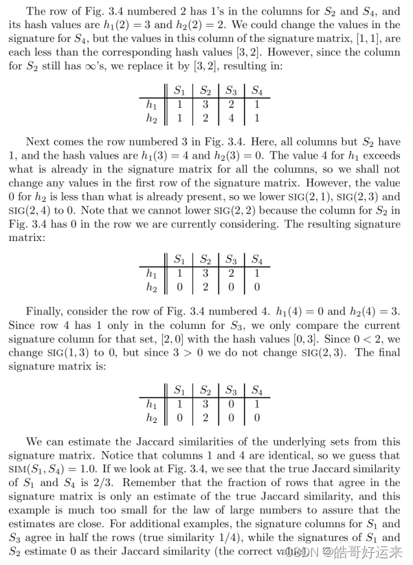
Our goal in this section is to replace large sets by much smaller representations called “signatures.” The important property we need for signatures is that we can compare the signatures of two sets and estimate the Jaccard similarity of the underlying sets from the signatures alone.
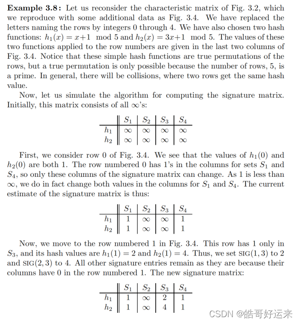
The signatures we desire to construct for sets are composed of the results of a large number of calculations, say several hundred, each of which is a “minhash” of the characteristic matrix.
To minhash a set represented by a column of the characteristic matrix, pick a permutation of the rows. The minhash value of any column is the number of the first row, in the permuted order, in which the column has a 1.
In this matrix, we can read off the values of h by scanning from the top until we come to a 1.
The probability that the minhash function for a random permutation of rows produces the same value for two sets equals the Jaccard similarity of those sets.
Call the minhash functions determined by these permutations
h
1
,
h
2
,
.
.
.
,
h
n
h_1, h_2, . . . , h_n
h1,h2,…,hn. From the column representing set S, construct the minhash signature for S, the
vector
[
h
1
(
S
)
,
h
2
(
S
)
,
.
.
.
,
h
n
(
S
)
]
[h_1(S), h_2(S), . . . , h_n(S)]
[h1(S),h2(S),…,hn(S)]. We normally represent this list of hash-values as a column. Thus, we can form from matrix M a signature matrix, in which the ith column of M is replaced by the minhash signature for (the set of) the ith column.
Moreover, the more minhashings we use, i.e., the more rows in the signature matrix, the smaller the expected error in the estimate of the Jaccard similarity will be.
Fortunately, it is possible to simulate the effect of a random permutation by a random hash function that maps row numbers to as many buckets as there are rows. A hash function that maps integers
0
,
1
,
.
.
.
,
k
−
1
0, 1, . . . , k − 1
0,1,…,k−1 to bucket numbers 0 through k−1 typically will map some pairs of integers to the same bucket and leave other buckets unfilled.
However, the difference is unimportant as long as k is large and there are not too many collisions. We can maintain the fiction that our hash function h “permutes” row r to position
h
(
r
)
h(r)
h(r) in the permuted order.
Thus, instead of picking n random permutations of rows, we pick n randomly chosen hash functions
h
1
,
h
2
,
.
.
.
,
h
n
h_1, h_2, . . . , h_n
h1,h2,…,hn on the rows. We construct the signature matrix by considering each row in their given order. Let
S
I
G
(
i
,
c
)
SIG(i, c)
SIG(i,c) be the element of the signature matrix for the ith hash function and column c. Initially, set
S
I
G
(
i
,
c
)
SIG(i, c)
SIG(i,c) to ∞ for all i and c. We handle row r by doing the following:
- Compute
h
1
(
r
)
,
h
2
(
r
)
,
.
.
.
,
h
n
(
r
)
h_1(r), h_2(r), . . . , h_n(r)
h1(r),h2(r),…,hn(r). - For each column c do the following:
(a) If c has 0 in row r, do nothing.
(b) However, if c has 1 in row r, then for eachi
=
1
,
2
,
.
.
.
,
n
i = 1, 2, . . . , n
i=1,2,…,n setS
I
G
(
i
,
c
)
SIG(i, c)
SIG(i,c) to the smaller of the current value ofS
I
G
(
i
,
c
)
SIG(i, c)
SIG(i,c) andh
i
(
r
)
h_i(r)
hi(r).
Example
The process of minhashing is time-consuming, since we need to examine the entire k-row matrix M for each minhash function we want.
But to compute one minhash function on all the columns, we shall not go all the way to the end of the permutation, but only look at the first m out of k rows. If we make m small compared with k, we reduce the work by a large factor, k/m.
However, there is a downside to making m small. As long as each column has at least one 1 in the first m rows in permuted order, the rows after the mth have no effect on any minhash value and may as well not be looked at.
But what if some columns are all-0’s in the first m rows? We have no minhash value
for those columns, and will instead have to use a special symbol, for which we
shall use ∞.
When we examine the minhash signatures of two columns in order to estimate the Jaccard similarity of their underlying sets, we have to take into account the possibility that one or both columns have ∞ as their minhash value for some components of the signature. There are three cases:
- If neither column has ∞ in a given row, then there is no change needed. Count this row as an example of equal values if the two values are the same, and as an example of unequal values if not.
- One column has ∞ and the other does not. In this case, had we used all the rows of the original permuted matrix M, the column that has the ∞ would eventually have been given some row number, and that number will surely not be one of the first m rows in the permuted order. But the other column does have a value that is one of the first m rows. Thus, we surely have an example of unequal minhash values, and we count this row of the signature matrix as such an example.
- Suppose both columns have ∞ in row. Then in the original permuted matrix M, the first m rows of both columns were all 0’s. We thus have no information about the Jaccard similarity of the corresponding sets; that similarity is only a function of the last
k
−
m
k − m
k−m rows, which we have chosen not to look at. We therefore count this row of the signature matrix as neither an example of equal values nor of unequal values.
As long as the third case, where both columns have ∞, is rare, we get almost as many examples to average as there are rows in the signature matrix. That effect will reduce the accuracy of our estimates of the Jaccard distance somewhat, but not much. And since we are now able to compute minhash values for all the columns much faster than if we examined all the rows of M, we can afford the time to apply a few more minhash functions. We get even better accuracy than originally, and we do so faster than before.
Suppose T is the set of elements of the universal set that are represented by the first m rows of matrix M. Let
S
1
S_1
S1 and
S
2
S_2
S2 be the sets represented by two columns of M. Then the first m rows of M represent the sets S1 ∩ T and S2 ∩ T . If both these sets are empty (i.e., both columns are all-0 in their first m rows), then this minhash function will be ∞ in both columns and will be ignored when estimating the Jaccard similarity of the columns’ underlying sets.
If at least one of the sets S1 ∩ T and S2 ∩ T is nonempty, then the probability of the two columns having equal values for this minhash function is the Jaccard similarity of these two sets, that is
∣
S
1
∩
S
2
∩
T
∣
∣
(
S
1
∪
S
2
)
∩
T
∣
frac{|S_1 ∩ S_2∩T|}{|(S_1cup S_2)cap T|}
∣(S1∪S2)∩T∣∣S1∩S2∩T∣
As long as T is chosen to be a random subset of the universal set, the expected value of this fraction will be the same as the Jaccard similarity of
S
1
S_1
S1 and
S
2
S_2
S2 However, there will be some random variation, since depending on T , we could find more or less than an average number of type X rows (1’s in both columns) and/or type Y rows (1 in one column and 0 in the other) among the first m rows of matrix M.
To mitigate this variation, we do not use the same set T for each minhashing that we do. Rather, we divide the rows of M into
k
/
m
k/m
k/m groups. Then for each hash function, we compute one minhash value by examining only the first m rows of M, a different minhash value by examining only the second m rows, and so on. We thus get
k
/
m
k/m
k/m minhash values from a single hash function and a single pass over all the rows of M. In fact, if
k
/
m
k/m
k/m is large enough, we may get all the rows of the signature matrix that we need by a single hash function applied to each of the subsets of rows of M.
Locality-Sensitive Hashing for Documents
One general approach to LSH is to “hash” items several times, in such a way that similar items are more likely to be hashed to the same bucket than dissimilar items are. We then consider any pair that hashed to the same bucket for any of the hashings to be a candidate pair. We check only the candidate pairs for similarity. The hope is that most of the dissimilar pairs will never hash to the same bucket, and therefore will never be checked. Those dissimilar pairs that do hash to the same bucket are false positives; we hope these will be only a small fraction of all pairs. We also hope that most of the truly similar pairs will hash to the same bucket under at least one of the hash functions. Those that do not are false negatives; we hope these will be only a small fraction of the truly similar pairs.
If we have minhash signatures for the items, an effective way to choose the hashings is to divide the signature matrix into b bands consisting of r rows each. For each band, there is a hash function that takes vectors of r integers (the portion of one column within that band) and hashes them to some large number of buckets. We can use the same hash function for all the bands, but we use a separate bucket array for each band, so columns with the same vector in different bands will not hash to the same bucket.
Suppose we use b bands of r rows each, and suppose that a particular pair of documents have Jaccard similarity s. The probability the minhash signatures for these documents agree in any one particular row of the signature matrix is s. We can calculate the probability that these documents (or rather their signatures) become a candidate pair as follows:
- The probability that the signatures agree in all rows of one particular band is
s
r
s^r
sr. - The probability that the signatures disagree in at least one row of a particular band is
1
−
s
r
1-s^r
1−sr. - The probability that the signatures disagree in at least one row of each of the bands is
(
1
−
s
r
)
b
(1-s^r)^b
(1−sr)b - The probability that the signatures agree in all the rows of at least one band, and therefore become a candidate pair, is
1
−
(
1
−
s
r
)
b
1-(1-s^r)^b
1−(1−sr)b.
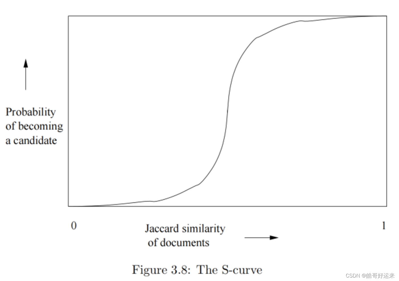
It may not be obvious, but regardless of the chosen constants b and r, this function has the form of an S-curve.
We can now give an approach to finding the set of candidate pairs for similar documents and then discovering the truly similar documents among them. It must be emphasized that this approach can produce false negatives – pairs of similar documents that are not identified as such because they never become a candidate pair. There will also be false positives – candidate pairs that are evaluated, but are found not to be sufficiently similar.
- Pick a value of k and construct from each document the set of k-shingles. Optionally, hash the k-shingles to shorter bucket numbers.
- Sort the document-shingle pairs to order them by shingle.
- Pick a length n for the minhash signatures. Feed the sorted list to the algorithm to compute the minhash signatures for all the documents.
- Choose a threshold t that defines how similar documents have to be in order for them to be regarded as a desired “similar pair.” Pick a number of bands b and a number of rows r such that
b
r
=
n
br = n
br=n, and the threshold t is approximately(
1
/
b
)
1
/
r
(1/b) ^{1/r}
(1/b)1/r. If avoidance of false negatives is important, you may wish to select b and r to produce a threshold lower than t; if speed is important and you wish to limit false positives, select b and r to produce a higher threshold. - Construct candidate pairs by applying the LSH technique.
- Examine each candidate pair’s signatures and determine whether the fraction of components in which they agree is at least t.
- Optionally, if the signatures are sufficiently similar, go to the documents themselves and check that they are truly similar, rather than documents that, by luck, had similar signatures
The LSH technique developed is one example of a family of functions (the minhash functions) that can be combined (by the banding technique) to distinguish strongly between pairs at a low distance from pairs at a high distance. The steepness of the S-curve in Fig. 3.8 reflects how effectively we can avoid false positives and false negatives among the candidate pairs. Now, we shall explore other families of functions, besides the minhash functions, that can serve to produce candidate pairs efficiently. These functions can apply to the space of sets and the Jaccard distance, or to another space and/or another distance measure. There are three conditions that we need for a family of functions:
- They must be more likely to make close pairs be candidate pairs than distant pairs.
- They must be statistically independent, in the sense that it is possible to estimate the probability that two or more functions will all give a certain response by the product rule for independent events.
- They must be efficient, in two ways:
(a) They must be able to identify candidate pairs in time much less than the time it takes to look at all pairs. For example, minhash functions have this capability, since we can hash sets to minhash values in time proportional to the size of the data, rather than the square of the number of sets in the data. Since sets with common values are colocated in a bucket, we have implicitly produced the candidate pairs for a single minhash function in time much less than
the number of pairs of sets.
(b) They must be combinable to build functions that are better at avoiding false positives and negatives, and the combined functions must also take time that is much less than the number of pairs. For example, the banding technique takes single minhash functions, which satisfy condition 3a but do not, by themselves have the S-curve behavior we want, and produces from a number of minhash functions a combined function that has the S-curve shape.
Locality-Sensitive Functions
For the purposes of this section, we shall consider functions that take two items and render a decision about whether these items should be a candidate pair.
In many cases, the function f will “hash” items, and the decision will be based on whether or not the result is equal. Because it is convenient to use the notation
f
(
x
)
=
f
(
y
)
f(x) = f(y)
f(x)=f(y) to mean that f(x, y) is “yes; make x and y a candidate pair,” we shall use
f
(
x
)
=
f
(
y
)
f(x) = f(y)
f(x)=f(y) as a shorthand with this meaning. We also use
f
(
x
)
≠
f
(
y
)
f(x) not = f(y)
f(x)=f(y) to mean “do not make x and y a candidate pair unless some other function concludes we should do so.”
A collection of functions of this form will be called a family of functions.
For example, the family of minhash functions, each based on one of the possible permutations of rows of a characteristic matrix, form a family.
Let
d
1
<
d
2
d_1 < d_2
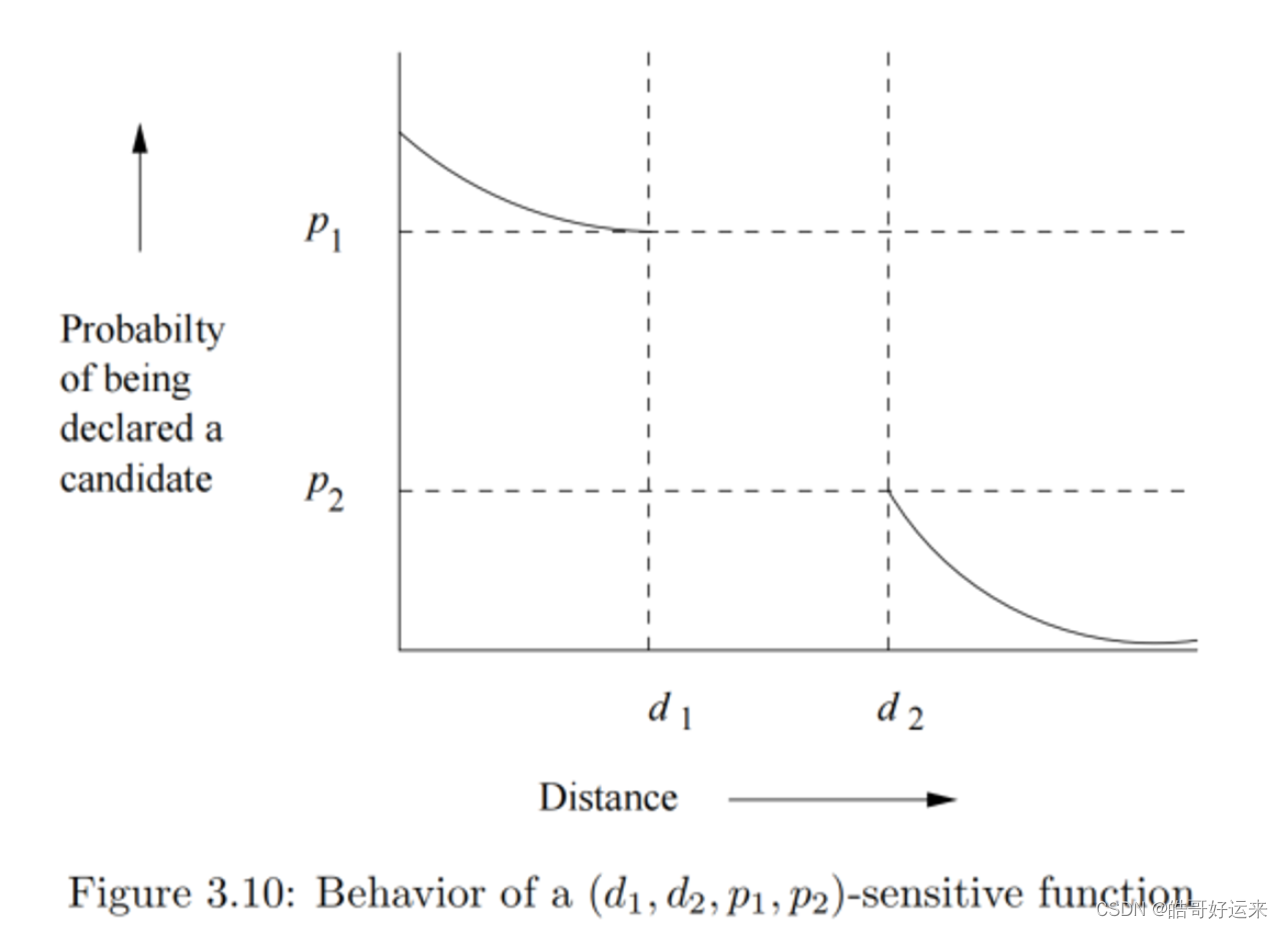
d1<d2 be two distances according to some distance measure d. A family F of functions is said to be (d1, d2, p1, p2)-sensitive if for every f in F:
- If
d
(
x
,
y
)
≤
d
1
d(x, y) ≤ d_1
d(x,y)≤d1, then the probability that f(x) = f(y) is at leastp
1
p_1
p1. - If
d
(
x
,
y
)
≥
d
2
d(x, y) ≥ d_2
d(x,y)≥d2, then the probability that f(x) = f(y) is at mostp
2
p_2
p2.
Suppose we are given a (d1, d2, p1, p2)-sensitive family F. We can construct a new family F′ by the AND-construction on F, which is defined as follows. Each member of F′ consists of r members of F for some fixed r. If f is in F′, and f is constructed from the set
f
1
,
f
2
,
.
.
.
,
f
r
{f_1, f_2, . . . , f_r}
f1,f2,…,fr of members of F, we say f(x) = f(y) if and only if
f
i
(
x
)
=
f
i
(
y
)
f_i(x) = f_i(y)
fi(x)=fi(y) for all i = 1, 2, . . . , r. Notice that this construction mirrors the effect of the r rows in a single band: the band makes x and y a candidate pair if every one of the r rows in the band say that x and y are equal (and therefore a candidate pair according to that row).
Since the members of F are independently chosen to make a member of F′, we can assert that F′ is a
(
d
1
,
d
2
,
(
p
1
)
r
,
(
p
2
)
r
)
(d_1,d_2,(p_1)^r,(p_2)^r)
(d1,d2,(p1)r,(p2)r) – sensitive family. That is, for any p, if p is the probability that a member of F will declare (x, y) to be a candidate pair, then the probability that a member of F′ will so declare is
p
r
p^r
pr.
There is another construction, which we call the OR-construction, that turns
a (d1, d2, p1, p2)-sensitive family F into a
(
d
1
,
d
2
,
1
−
(
1
−
p
1
)
b
,
1
−
(
1
−
p
2
)
b
)
(d_1,d_2,1-(1-p_1)^b,1-(1-p_2)^b)
(d1,d2,1−(1−p1)b,1−(1−p2)b)
sensitive family F′. Each member f of F′ is constructed from b members of F, say
f
1
,
f
2
,
.
.
.
,
f
b
f_1, f_2, . . . , f_b
f1,f2,…,fb. We define f(x) = f(y) if and only if
f
i
(
x
)
=
f
i
(
y
)
f_i(x) = f_i(y)
fi(x)=fi(y) for one or more values of i. The OR-construction mirrors the effect of combining several bands: x and y become a candidate pair if any band makes them a candidate pair.
Summary of Chapter 3
- Jaccard Similarity: The Jaccard similarity of sets is the ratio of the size of the intersection of the sets to the size of the union. This measure of similarity is suitable for many applications, including textual similarity of documents and similarity of buying habits of customers.
- Shingling: A k-shingle is any k characters that appear consecutively in a document. If we represent a document by its set of k-shingles, then the Jaccard similarity of the shingle sets measures the textual similarity of documents. Sometimes, it is useful to hash shingles to bit strings of shorter length, and use sets of hash values to represent documents.
- Minhashing: A minhash function on sets is based on a permutation of the universal set. Given any such permutation, the minhash value for a set is that element of the set that appears first in the permuted order.
- Minhash Signatures: We may represent sets by picking some list of permutations and computing for each set its minhash signature, which is the sequence of minhash values obtained by applying each permutation on the list to that set. Given two sets, the expected fraction of the permutations that will yield the same minhash value is exactly the Jaccard similarity of the sets.
- Efficient Minhashing: Since it is not really possible to generate random permutations, it is normal to simulate a permutation by picking a random hash function and taking the minhash value for a set to be the least hash value of any of the set’s members. An additional efficiency can be had by restricting the search for the smallest minhash value to only a small subset of the universal set.
- Locality-Sensitive Hashing for Signatures: This technique allows us to avoid computing the similarity of every pair of sets or their minhash signatures. If we are given signatures for the sets, we may divide them into bands, and only measure the similarity of a pair of sets if they are identical in at least one band. By choosing the size of bands appropriately, we can eliminate from consideration most of the pairs that do not meet our threshold of similarity.
- Distance Measures: A distance measure is a function on pairs of points in a space that satisfy certain axioms. The distance between two points is 0 if the points are the same, but greater than 0 if the points are different. The distance is symmetric; it does not matter in which order we consider the two points. A distance measure must satisfy the triangle inequality: the distance between two points is never more than the sum of the distances between those points and some third point.
- Euclidean Distance: The most common notion of distance is the Euclidean distance in an n-dimensional space. This distance, sometimes called the L2-norm, is the square root of the sum of the squares of the differences between the points in each dimension. Another distance suitable for Euclidean spaces, called Manhattan distance or the L1-norm is the sum of the magnitudes of the differences between the points in each dimension.
- Jaccard Distance: One minus the Jaccard similarity is a distance measure, called the Jaccard distance.
- Cosine Distance: The angle between vectors in a vector space is the cosine distance measure. We can compute the cosine of that angle by taking the dot product of the vectors and dividing by the lengths of the vectors.
- Edit Distance: This distance measure applies to a space of strings, and is the number of insertions and/or deletions needed to convert one string into the other. The edit distance can also be computed as the sum of the lengths of the strings minus twice the length of the longest common subsequence of the strings.
- Hamming Distance: This distance measure applies to a space of vectors. The Hamming distance between two vectors is the number of positions in which the vectors differ.
- Generalized Locality-Sensitive Hashing: We may start with any collection of functions, such as the minhash functions, that can render a decision as to whether or not a pair of items should be candidates for similarity checking. The only constraint on these functions is that they provide a lower bound on the probability of saying “yes” if the distance (according to some distance measure) is below a given limit, and an upper bound on the probability of saying “yes” if the distance is above another given limit. We can then increase the probability of saying “yes” for nearby items and at the same time decrease the probability of saying “yes” for distant items to as great an extent as we wish, by applying an AND construction and an OR construction.
- Random Hyperplanes and LSH for Cosine Distance: We can get a set of basis functions to start a generalized LSH for the cosine distance measure by identifying each function with a list of randomly chosen vectors. We apply a function to a given vector v by taking the dot product of v with each vector on the list. The result is a sketch consisting of the signs (+1 or −1) of the dot products. The fraction of positions in which the sketches of two vectors agree, multiplied by 180, is an estimate of the angle between the two vectors.
- LSH For Euclidean Distance: A set of basis functions to start LSH for Euclidean distance can be obtained by choosing random lines and projecting points onto those lines. Each line is broken into fixed–length intervals, and the function answers “yes” to a pair of points that fall into the same interval.
- High-Similarity Detection by String Comparison: An alternative approach to finding similar items, when the threshold of Jaccard similarity is close to 1, avoids using minhashing and LSH. Rather, the universal set is ordered, and sets are represented by strings, consisting their elements in order. The simplest way to avoid comparing all pairs of sets or their strings is to note that highly similar sets will have strings of approximately the same length. If we sort the strings, we can compare each string with only a small number of the immediately following strings.
- Character Indexes: If we represent sets by strings, and the similarity threshold is close to 1, we can index all strings by their first few characters. The prefix whose characters must be indexed is approximately the length of the string times the maximum Jaccard distance (1 minus the minimum Jaccard similarity).
- Position Indexes: We can index strings not only on the characters in their prefixes, but on the position of that character within the prefix. We reduce the number of pairs of strings that must be compared, because if two strings share a character that is not in the first position in both strings, then we know that either there are some preceding characters that are in the union but not the intersection, or there is an earlier symbol that appears in both strings.
- Suffix Indexes: We can also index strings based not only on the characters in their prefixes and the positions of those characters, but on the length of the character’s suffix – the number of positions that follow it in the string. This structure further reduces the number of pairs that must be compared, because a common symbol with different suffix lengths implies additional characters that must be in the union but not in the intersection.
END
ps. 终于看完了,下一本书跨专业咯:《营销管理》(第15版)
原文地址:https://blog.csdn.net/qq_52370024/article/details/134618645
本文来自互联网用户投稿,该文观点仅代表作者本人,不代表本站立场。本站仅提供信息存储空间服务,不拥有所有权,不承担相关法律责任。
如若转载,请注明出处:http://www.7code.cn/show_12553.html
如若内容造成侵权/违法违规/事实不符,请联系代码007邮箱:suwngjj01@126.com进行投诉反馈,一经查实,立即删除!


![[数据挖掘、数据分析] clickhouse在go语言里的实践](https://img-blog.csdnimg.cn/33371cb205b14839a4fd8f047f509b7f.png)
