PyTorch|构建自己的卷积神经网络

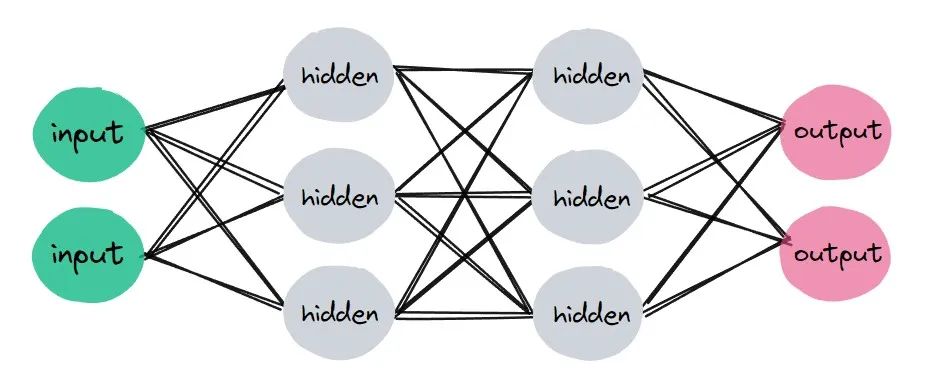
本文介绍: 如何搭建网络，这在深度学习中非常重要。简单来讲，我们是要实现一个类，这个类中有属性和方法，能够进行计算。一般来讲，使用PyTorch创建神经网络需要三步：继承基类：nn.Module定义层属性实现前向传播方法

如何搭建网络，这在深度学习中非常重要。简单来讲，我们是要实现一个类，这个类中有属性和方法，能够进行计算。

一般来讲，使用PyTorch创建神经网络需要三步：

继承基类：nn.Module
定义层属性
实现前向传播方法

如果你对于python面向对象编程非常熟练，那么这里也就非常简单，就是定义一些属性，实现一些方法。

开始建立一个网络，就像这样：

import torchimport torch.nn as nnimport torch.nn.functional as Fclass Network(nn.Module):    def __init__(self):        super(Network, self).__init__()        self.conv1 = nn.Conv2d(in_channels=1, out_channels=6, kernel_size=5)        self.conv2 = nn.Conv2d(in_channels=6, out_channels=12, kernel_size=5)        self.fc1 = nn.Linear(in_features=12*4*4, out_features=120)        self.fc2 = nn.Linear(in_features=120,out_features=60)        self.out = nn.Linear(in_features=60, out_features=10)    def forward(self,t):        # (1) input layer        t = t        # (2) hidden conv layer1        t = self.conv1(t)        t = F.relu(t)        t = F.max_pool2d(t, kernel_size=2, stride=2)        # (3) hidden conv layer2        t = self.conv2(t)        t = F.relu(t)        t = F.max_pool2d(t, kernel_size=2, stride=2)        # relu 和 max pooling 都没有权重；激活层和池化层的本质都是对传入的数据按照一定的算法变换。        #（4）hidden linear layer2        t = t.reshape(-1, 12*4*4)        t = self.fc1(t)        t = F.relu(t)        # (5) hidden linear layer2        t = self.fc2(t)        t = F.relu(t)        # (6) output layer        t = self.out(t)

对于上述代码，就是定义了一个新的类，叫做Network,这个类继承自nn.Module,同时，我们又新定义了一些属性，比如conv1,conv2,fc1,fc2,out，并实现了一个方法，叫做：forawrd。

好吧，接下来我们进行初始化

>>>network=Network()

访问对象network的一些属性

>>> network.conv1Conv2d(1, 6, kernel_size=(5, 5), stride=(1, 1))>>> network.conv2Conv2d(6, 12, kernel_size=(5, 5), stride=(1, 1))>>> network.outLinear(in_features=60, out_features=10, bias=True)

更进一步，我们也可获得每一层的权重，形状：

>>> network.conv2.weightParameter containing:tensor([[[[-8.0741e-02, -7.1281e-02,  7.6540e-02,  6.2786e-02,  1.1018e-03],          [ 6.5041e-02, -3.5665e-02,  7.8475e-02, -1.1228e-02, -2.9447e-02],          [-8.0508e-02,  7.0457e-02,  7.7877e-02,  7.2872e-02,  4.5671e-02],          [ 3.9757e-03,  7.7676e-02,  3.3951e-02,  6.3745e-02,  7.0577e-02],          [-2.0165e-02,  2.2356e-02,  2.9137e-02,  8.0388e-02,  5.9048e-02]]............>>> network.conv2.weight.shapetorch.Size([12, 6, 5, 5])

好吧，上述操作比较繁琐，我们不想这样做，但我们还是非常想了解一个神经网络，那么应该怎么办呢？其实，可以这样。

好吧，接下来我们进行初始化

>>>network=Network()>>> networkNetwork(  (conv1): Conv2d(1, 6, kernel_size=(5, 5), stride=(1, 1))  (conv2): Conv2d(6, 12, kernel_size=(5, 5), stride=(1, 1))  (fc1): Linear(in_features=192, out_features=120, bias=True)  (fc2): Linear(in_features=120, out_features=60, bias=True)  (out): Linear(in_features=60, out_features=10, bias=True))
>>> for name, param in network.named_parameters():    print(name,'tt', param.shape)    conv1.weight      torch.Size([6, 1, 5, 5])conv1.bias      torch.Size([6])conv2.weight      torch.Size([12, 6, 5, 5])conv2.bias      torch.Size([12])fc1.weight      torch.Size([120, 192])fc1.bias      torch.Size([120])fc2.weight      torch.Size([60, 120])fc2.bias      torch.Size([60])out.weight      torch.Size([10, 60])out.bias      torch.Size([10])

我们实现的新的类是基于基类nn.Module实现的，nn.Linear(in_features=120, out_features=60)是一个线性层，是PyTorch已经实现好的。主要功能就是我们输入一个数据，这个层对数据进行一个线性变换，最后输出一个数据。

还记得之前我们获得了神经网络各层的权重尺寸：

>>> network.fc2.weight.shapetorch.Size([60, 120])

没错，是一个60×120的矩阵。

一个1×120的数据，进入线性层，经过线性变换，最后变成形状为1×60的矩阵。当然，这里解释不是非常正确，Linear层复杂得多，这里仅仅是为了便于理解。

如果你还不理解，下面这个例子可能更加简单：

# 1. 张量的乘法in_features = torch.tensor([1,2,3,4], dtype=torch.float32)weight_matrix = torch.tensor([    [1,2,3,4],    [2,3,4,5],    [3,4,5,6]], dtype = torch.float32)result1=weight_matrix.matmul(in_features)# 可将上述的权重矩阵看作是一个线性映射.
# 在parameter类中包装一个权重矩阵，以使得输出结果与1中一样fc = nn.Linear(in_features=4, out_features=3)fc.weight= nn.Parameter(weight_matrix)result2=fc(in_features)# 此时的结果接近1中的结果却不精确，是因为由bias的存在
>>> print(result1)tensor([30., 40., 50.])>>> print(result2)tensor([29.5786, 39.9564, 49.7925], grad_fn=<AddBackward0>)