本文介绍: AdaBoost的基本思想是对训练样本进行加权,将分类错误的样本权值增大,再训练下一个分类器。经过多轮迭代,每个样本都会得到不同的权值,并且每个分类器都有一定的权重。最终,AdaBoost通过对所有分类器的加权求和,得到最终的分类结果。它通过训练一系列弱分类器(即准确率略高于随机猜测的分类器),然后将它们组合成一个强分类器。总的来说,AdaBoost是一种强大的集成学习算法,可以通过组合多个弱分类器来提高分类的准确性。最终的强分类器是将每个弱分类器的输出加权求和,并根据总体输出判断样本的分类。
目录
4.7用RandomForestRegressor预测年龄填补缺失数据
介绍:
AdaBoost(Adaptive Boosting)是一种集成学习方法,用于提高机器学习算法的准确性。它通过训练一系列弱分类器(即准确率略高于随机猜测的分类器),然后将它们组合成一个强分类器。
AdaBoost的基本思想是对训练样本进行加权,将分类错误的样本权值增大,再训练下一个分类器。经过多轮迭代,每个样本都会得到不同的权值,并且每个分类器都有一定的权重。最终,AdaBoost通过对所有分类器的加权求和,得到最终的分类结果。
在AdaBoost中,每个弱分类器的训练过程如下:
- 初始化样本权值为相等值。
- 使用权值训练一个弱分类器。
- 根据分类错误率计算该分类器的权重。
- 更新样本权值,增加分类错误的样本权值,并减小分类正确的样本权值。
- 重复步骤2到4,直到达到指定的弱分类器个数或达到某个条件。
最终的强分类器是将每个弱分类器的输出加权求和,并根据总体输出判断样本的分类。
AdaBoost模型有一些特点:
- 适用于二分类和多分类问题。
- 对于弱分类器的选择没有严格的限制,可以使用任何分类器作为基分类器。
- 在训练过程中,每个样本都被赋予不同的权重,以便更加关注错误分类的样本。
- 可以减少过拟合问题,因为它将注意力集中在难以分类的样本上。
- AdaBoost的训练速度较快,预测速度也较快。
总的来说,AdaBoost是一种强大的集成学习算法,可以通过组合多个弱分类器来提高分类的准确性。它在实际应用中取得了很好的效果,并广泛应用于各个领域。
二、数据
2.1引用数据
import pandas as pd
import numpy as np
import matplotlib.pyplot as plt
import seaborn as sns
%matplotlib inline

import warnings
warnings.filterwarnings('ignore')##忽略警告

train = pd.read_csv("train.csv")
test = pd.read_csv("test.csv")

passengerid = test.PassengerId

print(train.info())
print('*'*80)
print(test.info())
'''结果:
<class 'pandas.core.frame.DataFrame'>
RangeIndex: 891 entries, 0 to 890
Data columns (total 12 columns):
 #   Column       Non-Null Count  Dtype
---  ------       --------------  -----
 0   PassengerId  891 non-null    int64
 1   Survived     891 non-null    int64
 2   Pclass       891 non-null    int64
 3   Name         891 non-null    object
 4   Sex          891 non-null    object
 5   Age          714 non-null    float64
 6   SibSp        891 non-null    int64
 7   Parch        891 non-null    int64
 8   Ticket       891 non-null    object
 9   Fare         891 non-null    float64
 10  Cabin        204 non-null    object
 11  Embarked     889 non-null    object
dtypes: float64(2), int64(5), object(5)
memory usage: 83.7+ KB
None
********************************************************************************
<class 'pandas.core.frame.DataFrame'>
RangeIndex: 418 entries, 0 to 417
Data columns (total 12 columns):
 #   Column       Non-Null Count  Dtype
---  ------       --------------  -----
 0   PassengerId  418 non-null    int64
 1   Survived     418 non-null    int64
 2   Pclass       418 non-null    int64
 3   Name         418 non-null    object
 4   Sex          418 non-null    object
 5   Age          332 non-null    float64
 6   SibSp        418 non-null    int64
 7   Parch        418 non-null    int64
 8   Ticket       418 non-null    object
 9   Fare         417 non-null    float64
 10  Cabin        91 non-null     object
 11  Embarked     418 non-null    object
dtypes: float64(2), int64(5), object(5)
memory usage: 39.3+ KB
None
'''
2.2检查缺失数据
2.2.1手动检查缺失数据
def missing_percentage(df):#显示空缺数据
    total = df.isnull().sum().sort_values(ascending=False)
    percent = round(df.isnull().sum().sort_values(ascending=False)/len(df)*100,2)
    return pd.concat([total,percent],axis=1,keys=['Total','Percent'])

missing_percentage(train)#检查缺失数据
'''结果:
 	Total 	Percent
Cabin 	687 	77.10
Age 	177 	19.87
Embarked 	2 	0.22
PassengerId 	0 	0.00
Survived 	0 	0.00
Pclass 	0 	0.00
Name 	0 	0.00
Sex 	0 	0.00
SibSp 	0 	0.00
Parch 	0 	0.00
Ticket 	0 	0.00
Fare 	0 	0.00
'''

missing_percentage(test)
'''结果:
 	Total 	Percent
Cabin 	327 	78.23
Age 	86 	20.57
Fare 	1 	0.24
PassengerId 	0 	0.00
Survived 	0 	0.00
Pclass 	0 	0.00
Name 	0 	0.00
Sex 	0 	0.00
SibSp 	0 	0.00
Parch 	0 	0.00
Ticket 	0 	0.00
Embarked 	0 	0.00
'''
def percent_value_counts(df,feature):#统计一个特征值的特征类别
percent = pd.DataFrame(round(df.loc[:,feature].value_counts(dropna=False,normalize=True)*100,2))
total = pd.DataFrame(df.loc[:,feature].value_counts(dropna=False))
total.columns=["Total"]
percent.columns=['Percent']
return pd.concat([total,percent],axis=1)
percent_value_counts(train,'Embarked')
'''结果:
Total Percent
S 644 72.28
C 168 18.86
Q 77 8.64
NaN 2 0.22
'''2.2.2查看某一个特征值为空数据
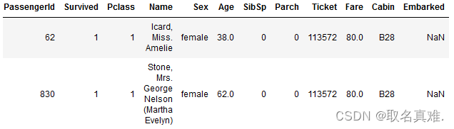
train[train.Embarked.isnull()]#查看某一特征值为空的数据
2.3补充缺失数据
2.3.1盒图
sns.set_style('darkgrid')
fig, ax = plt.subplots(figsize=(16,12),ncols=2)#前面表示图的大小,后面表示两个图

ax1 = sns.boxplot(x="Embarked", y="Fare", hue="Pclass", data=train, ax = ax[0]);
ax2 = sns.boxplot(x="Embarked", y="Fare", hue="Pclass", data=test,ax = ax[1]);

ax1.set_title("Training set", fontsize=18)
ax2.set_title('Test set', fontsize=18)

## Fixing Legends
leg_1 = ax1.get_legend()
leg_1.set_title("PClass")
legs = leg_1.texts
legs[0].set_text('upper')
legs[1].set_text('Middle')
legs[2].set_text('Lower')

fig.show( )#可以看均值,通过均值补充空的值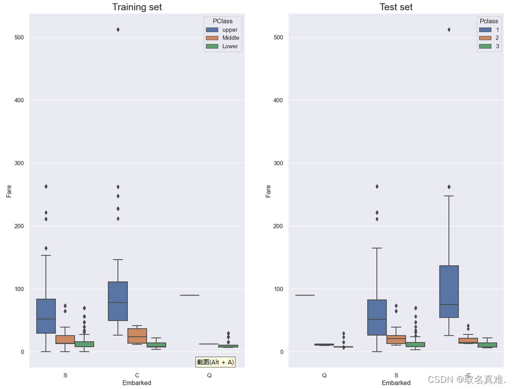
train.Embarked.fillna("C",inplace=True)#填充空数据

##缺失数据的Pclass为1,票价为80,根据盒图可以看出Pclass为1,票价均值为80的c
#所以用c补充数据
2.3.2手动用均值填补缺失数据
print("Train Cabin missing:" + str(train.Cabin.isnull().sum()/len(train.Cabin)))
#结果:Train Cabin missing:0.7710437710437711

'''缺失数据量大,把训练集和测试集合并'''
survivers = train.Survived
train.drop(["Survived"],axis=1, inplace=True)

all_data = pd.concat([train,test],ignore_index=False)#train和test连接起来

#* Assign all the null values to N
all_data.Cabin.fillna("N", inplace=True)#先用N补充空数据


percent_value_counts(all_data,"Cabin")#统计一个特征值的特征个数
'''结果:
 	Total 	Percent
N 	1014 	77.46
C 	94 	    7.18
B 	65 	    4.97
D 	46 	    3.51
E 	41 	    3.13
A 	22 	    1.68
F 	21 	    1.60
G 	5 	    0.38
T 	1 	    0.08
'''

all_data.groupby("Cabin")['Fare'].mean().sort_values()#每个舱位的票价均值
'''结果:
Cabin
G     14.205000
F     18.079367
N     19.132707
T     35.500000
A     41.244314
D     53.007339
E     54.564634
C    107.926598
B    122.383078
Name: Fare, dtype: float64
'''
def cabin_estimator(i):#"""grouping cabin feature by the first letter"""
a = 0
if i<16:
a="G"
elif i>=16 and i<27:
a="F"
elif i>=27 and i<38:
a="T"
elif i>=38 and i<47:
a="A"
elif i>= 47 and i<53:
a="E"
elif i>= 53 and i<54:
a="D"
elif i>=54 and i<116:
a='C'
else:
a="B"
return a
#把为N的挑出来,不为N挑出来
with_N = all_data[all_data.Cabin == "N"]
without_N = all_data[all_data.Cabin != "N"]
##opplying cabin estimator function.
with_N['Cabin'] = with_N.Fare.apply(lambda x: cabin_estimator(x))#根据票价赋值
## getting back train.
all_data = pd.concat([with_N, without_N],axis=0)#连接在一起
## PassengerId helps us separate train and test.
all_data.sort_values(by ='PassengerId', inplace=True)
## Separating train and test from all_data.
train = all_data[:891]#再分训练集和测试集
test = all_data[891:]
#adding saved target variable with train.
train['Survived']=survivers2.3.3手动用类别填补缺失数据
test[test.Fare.isnull()]
'''结果:
 	PassengerId 	Pclass 	Name 	Sex 	Age 	SibSp 	Parch 	Ticket 	Fare 	Cabin 	Embarked 	Survived
152 	1044 	3 	Storey, Mr. Thomas 	male 	60.5 	0 	0 	3701 	NaN 	B 	S 	0.0
'''

missing_value = test[(test.Pclass == 3)&
                     (test.Embarked == 'S')&
                     (test.Sex == 'male')].Fare.mean()#求这类乘客的票价均值

test.Fare.fillna(missing_value,inplace=True)#将均值赋给空
三、数据分析
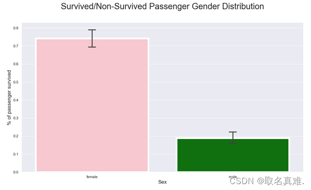
3.1男女生存比例
import seaborn as sns
pal = {'male':"green", 'female':"Pink"}
sns.set(style="darkgrid")
plt.subplots(figsize = (15,8))
ax = sns.barplot(x = "Sex",
                 y = "Survived",
                 data=train,
                 palette = pal,
                 linewidth=5,
                 order = ['female','male'],
                 capsize = .05,

                )

plt.title("Survived/Non-Survived Passenger Gender Distribution", fontsize = 25,loc = 'center', pad = 40)
plt.ylabel("% of passenger survived", fontsize = 15, )
plt.xlabel("Sex",fontsize = 15);
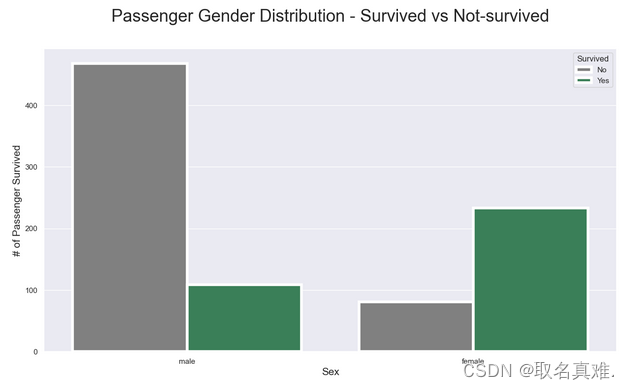
3.2男女生存数
pal = {1:"seagreen", 0:"gray"}
sns.set(style="darkgrid")
plt.subplots(figsize = (15,8))
ax = sns.countplot(x = "Sex",
                   hue="Survived",
                   data = train,
                   linewidth=4,
                   palette = pal
)

## Fixing title, xlabel and ylabel
plt.title("Passenger Gender Distribution - Survived vs Not-survived", fontsize = 25, pad=40)
plt.xlabel("Sex", fontsize = 15);
plt.ylabel("# of Passenger Survived", fontsize = 15)

## Fixing xticks
#labels = ['Female', 'Male']
#plt.xticks(sorted(train.Sex.unique()), labels)

## Fixing legends
leg = ax.get_legend()
leg.set_title("Survived")
legs = leg.texts
legs[0].set_text("No")
legs[1].set_text("Yes")
plt.show()
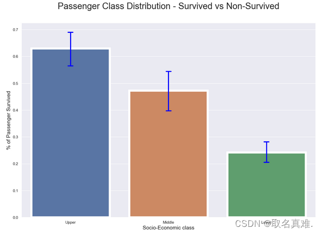
3.3船舱级别生存比例
plt.subplots(figsize = (15,10))
sns.barplot(x = "Pclass",
            y = "Survived",
            data=train,
            linewidth=6,
            capsize = .05,
            errcolor='blue',
            errwidth = 3


           )
plt.title("Passenger Class Distribution - Survived vs Non-Survived", fontsize = 25, pad=40)
plt.xlabel("Socio-Economic class", fontsize = 15);
plt.ylabel("% of Passenger Survived", fontsize = 15);
names = ['Upper', 'Middle', 'Lower']
#val = sorted(train.Pclass.unique())
val = [0,1,2] ## this is just a temporary trick to get the label right.
plt.xticks(val, names);
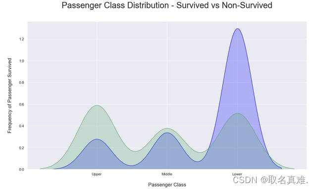
3.4船舱生存与死亡比例
# Kernel Density Plot
fig = plt.figure(figsize=(15,8),)
## I have included to different ways to code a plot below, choose the one that suites you.
ax=sns.kdeplot(train.Pclass[train.Survived == 0] ,
               color='blue',
               shade=True,
               label='not survived')
ax=sns.kdeplot(train.loc[(train['Survived'] == 1),'Pclass'] ,
               color='g',
               shade=True,
               label='survived',
              )
plt.title('Passenger Class Distribution - Survived vs Non-Survived', fontsize = 25, pad = 40)
plt.ylabel("Frequency of Passenger Survived", fontsize = 15, labelpad = 20)
plt.xlabel("Passenger Class", fontsize = 15,labelpad =20)
## Converting xticks into words for better understanding
labels = ['Upper', 'Middle', 'Lower']
plt.xticks(sorted(train.Pclass.unique()), labels);
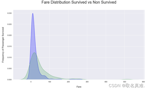
3.5票价与生存关系
# Kernel Density Plot
fig = plt.figure(figsize=(15,8),)
ax=sns.kdeplot(train.loc[(train['Survived'] == 0),'Fare'] , color='blue',shade=True,label='not survived')
ax=sns.kdeplot(train.loc[(train['Survived'] == 1),'Fare'] , color='g',shade=True, label='survived')
plt.title('Fare Distribution Survived vs Non Survived', fontsize = 25, pad = 40)
plt.ylabel("Frequency of Passenger Survived", fontsize = 15, labelpad = 20)
plt.xlabel("Fare", fontsize = 15, labelpad = 20);
3.6年龄与生存关系
# Kernel Density Plot
fig = plt.figure(figsize=(15,8),)
ax=sns.kdeplot(train.loc[(train['Survived'] == 0),'Age'] , color='blue',shade=True,label='not survived')
ax=sns.kdeplot(train.loc[(train['Survived'] == 1),'Age'] , color='g',shade=True, label='survived')
plt.title('Age Distribution - Surviver V.S. Non Survivors', fontsize = 25, pad = 40)
plt.xlabel("Age", fontsize = 15, labelpad = 20)
plt.ylabel('Frequency', fontsize = 15, labelpad= 20); 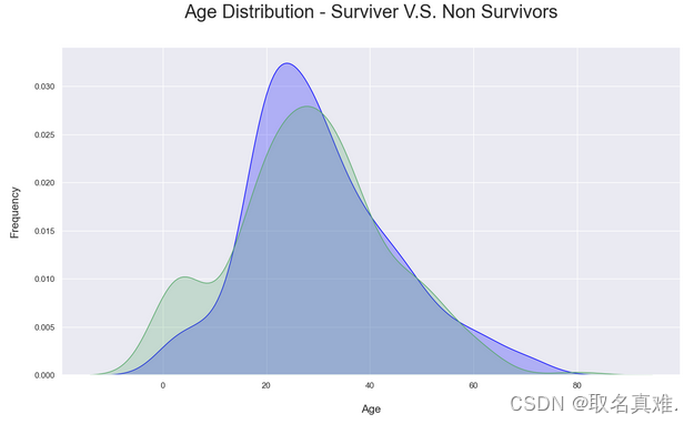
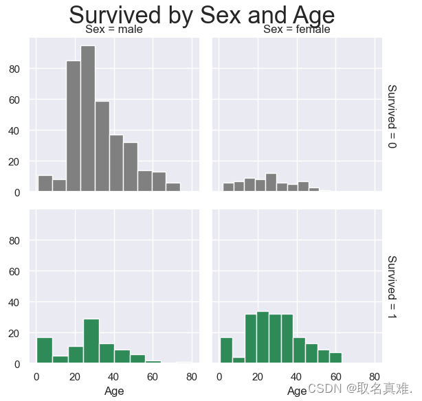
3.7性别年龄与生存关系
pal = {1:"seagreen", 0:"gray"}
g = sns.FacetGrid(train,  col="Sex", row="Survived", margin_titles=True, hue = "Survived",
                  palette=pal)
g = g.map(plt.hist, "Age", edgecolor = 'white');
g.fig.suptitle("Survived by Sex and Age", size = 25)
plt.subplots_adjust(top=0.90)
3.8性别、登口岸、年龄与生存关系
g = sns.FacetGrid(train, col="Sex", row="Embarked", margin_titles=True, hue = "Survived",
                  palette = pal
                  )
g = g.map(plt.hist, "Age", edgecolor = 'white').add_legend();
g.fig.suptitle("Survived by Sex and Age", size = 25)
plt.subplots_adjust(top=0.90)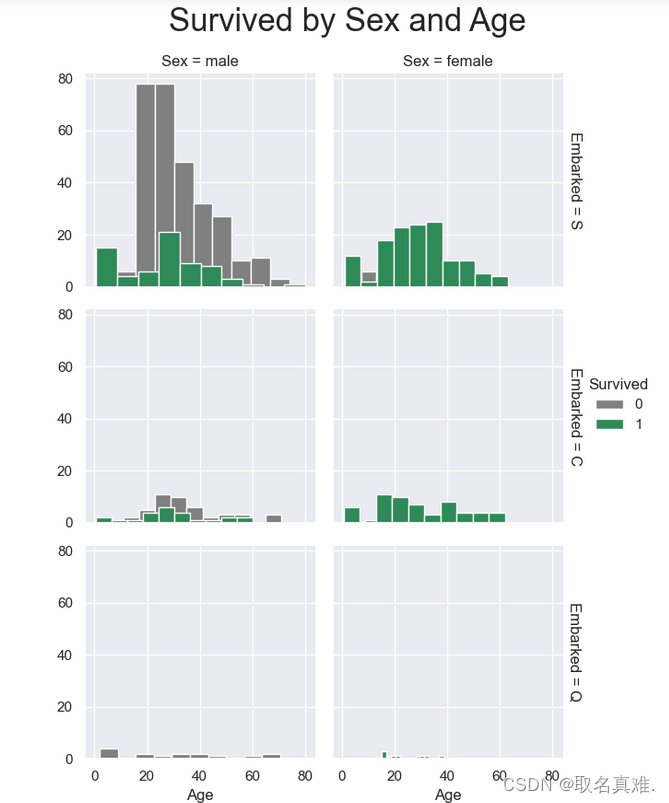
3.9性别、票价、年龄与生存关系
g = sns.FacetGrid(train,hue="Survived", col ="Sex", margin_titles=True,
                palette=pal,)
g.map(plt.scatter, "Fare", "Age",edgecolor="w").add_legend()
g.fig.suptitle("Survived by Sex, Fare and Age", size = 25)
plt.subplots_adjust(top=0.85) 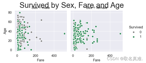
四、数据处理
4.1处理性别
male_mean = train[train['Sex'] == 1].Survived.mean()

female_mean = train[train['Sex'] == 0].Survived.mean()
print ("Male survival mean: " + str(male_mean))
print ("female survival mean: " + str(female_mean))

print ("The mean difference between male and female survival rate: " + str(female_mean - male_mean))

'''结果:
Male survival mean: 0.18890814558058924
female survival mean: 0.7420382165605095
The mean difference between male and female survival rate: 0.5531300709799203
'''

# separating male and female dataframe.
import random
male = train[train['Sex'] == 1]
female = train[train['Sex'] == 0]

## empty list for storing mean sample
m_mean_samples = []
f_mean_samples = []

for i in range(50):
    m_mean_samples.append(np.mean(random.sample(list(male['Survived']),50,)))
    f_mean_samples.append(np.mean(random.sample(list(female['Survived']),50,)))


# Print them out
print (f"Male mean sample mean: {round(np.mean(m_mean_samples),2)}")
print (f"Female mean sample mean: {round(np.mean(f_mean_samples),2)}")
print (f"Difference between male and female mean sample mean: {round(np.mean(f_mean_samples) - np.mean(m_mean_samples),2)}")


'''结果:
Male mean sample mean: 0.18
Female mean sample mean: 0.74
Difference between male and female mean sample mean: 0.56
'''
# Placing 0 for female and
# 1 for male in the "Sex" column.
train['Sex'] = train.Sex.apply(lambda x: 0 if x == "female" else 1)
test['Sex'] = test.Sex.apply(lambda x: 0 if x == "female" else 1)train.describe()#数据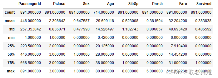
survived_summary = train.groupby("Survived")
survived_summary.mean().reset_index()
'''结果:
 	Survived 	PassengerId 	Pclass 	Sex 	Age 	SibSp 	Parch 	Fare
0 	0 	447.016393 	2.531876 	0.852459 	30.626179 	0.553734 	0.329690 	22.117887
1 	1 	444.368421 	1.950292 	0.318713 	28.343690 	0.473684 	0.464912 	48.395408
'''

survived_summary = train.groupby("Sex")
survived_summary.mean().reset_index()
'''结果:
 	Sex 	PassengerId 	Pclass 	Age 	SibSp 	Parch 	Fare 	Survived
0 	0 	431.028662 	2.159236 	27.915709 	0.694268 	0.649682 	44.479818 	0.742038
1 	1 	454.147314 	2.389948 	30.726645 	0.429809 	0.235702 	25.523893 	0.188908
'''

survived_summary = train.groupby("Pclass")
survived_summary.mean().reset_index()
'''结果:
 	Pclass 	PassengerId 	Sex 	Age 	SibSp 	Parch 	Fare 	Survived
0 	1 	461.597222 	0.564815 	38.233441 	0.416667 	0.356481 	84.154687 	0.629630
1 	2 	445.956522 	0.586957 	29.877630 	0.402174 	0.380435 	20.662183 	0.472826
2 	3 	439.154786 	0.706721 	25.140620 	0.615071 	0.393075 	13.675550 	0.242363
'''

pd.DataFrame(abs(train.corr()["Survived"]).sort_values(ascending=False))#相关性
'''结果:

 	Survived
Survived 	1.000000
Sex 	0.543351
Pclass 	0.338481
Fare 	0.257307
Parch 	0.081629
Age 	0.077221
SibSp 	0.035322
PassengerId 	0.005007
'''
4.2热图表相关性
corr = train.corr()**2
corr.Survived.sort_values(ascending = False)


## heatmeap to see the correlatton between features
# Generate a mask for the upper triangle (taken from seaborn example gallery)
import numpy as np
mask = np.zeros_like(train.corr(),dtype=bool)
mask[np.triu_indices_from(mask)]  = True
sns.set_style("whitegrid")

plt.subplots(figsize = (15,12))
sns.heatmap(train.corr(),
            annot=True,
            mask = mask,
            cmap = 'RdBu', ## in order to reverse the bar replace "RdBu" with "RdBur'
            linewidths=.9,
            linecolor="white",
             fmt='.2g',
            center = 0,
            square=True)
plt.title("correlations Among Features", y = 1.03,fontsize = 20, pad = 40);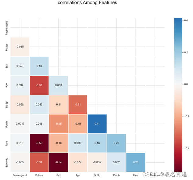
4.3姓名处理
# Creating a new colomn with a
train['name_length'] = [len(i) for i in train.Name]
test['name_length'] = [len(i) for i in test.Name]

def name_length_group(size):
    a = ''
    if (size <=20):
        a = 'short'
    elif (size <=35):
        a = 'medium'
    elif (size <=45):
        a = 'good'
    else:
        a = 'long'
    return a


train['nLength_group'] = train['name_length'].map(name_length_group)
test['nLength_group'] = test['name_length'].map(name_length_group)

## Here "map" is python's built-in function.
## "map" function basically takes a function and
## returns an iterable list/tuple or in this case series.
## However,"map" can also be used like map(function) e.g. map(name_length_group)
## or map(function, iterable{list, tuple}) e.g. map(name_length_group, train[feature]]).
## However, here we don't need to use parameter("size") for name_length_group because when we
## used the map function like ".map" with a series before dot, we are basically hinting that series
## and the iterable. This is similar to .append approach in python. list.append(a) meaning applying append on list.


## cuts the column by given bins based on the range of name_length
#group_names = ['short', 'medium', 'good', 'long']
#train['name_len_group'] = pd.cut(train['name_length'], bins = 4, labels=group_names)
## get the title from the name
train["title"] = [i.split('.')[0] for i in train.Name]
train["title"] = [i.split(',')[1] for i in train.title]
## Whenever we split like that, there is a good change that
#we will end up with white space around our string values. Let's check that.
print(train.title.unique())
'''结果:
[' Mr' ' Mrs' ' Miss' ' Master' ' Don' ' Rev' ' Dr' ' Mme' ' Ms' ' Major'
' Lady' ' Sir' ' Mlle' ' Col' ' Capt' ' the Countess' ' Jonkheer']
'''
## Let's fix that
train.title = train.title.apply(lambda x: x.strip())
## We can also combile all three lines above for test set here
test['title'] = [i.split('.')[0].split(',')[1].strip() for i in test.Name]
## However it is important to be able to write readable code, and the line above is not so readable.
## Let's replace some of the rare values with the keyword 'rare' and other word choice of our own.
## train Data
train["title"] = [i.replace('Ms', 'Miss') for i in train.title]
train["title"] = [i.replace('Mlle', 'Miss') for i in train.title]
train["title"] = [i.replace('Mme', 'Mrs') for i in train.title]
train["title"] = [i.replace('Dr', 'rare') for i in train.title]
train["title"] = [i.replace('Col', 'rare') for i in train.title]
train["title"] = [i.replace('Major', 'rare') for i in train.title]
train["title"] = [i.replace('Don', 'rare') for i in train.title]
train["title"] = [i.replace('Jonkheer', 'rare') for i in train.title]
train["title"] = [i.replace('Sir', 'rare') for i in train.title]
train["title"] = [i.replace('Lady', 'rare') for i in train.title]
train["title"] = [i.replace('Capt', 'rare') for i in train.title]
train["title"] = [i.replace('the Countess', 'rare') for i in train.title]
train["title"] = [i.replace('Rev', 'rare') for i in train.title]
## Now in programming there is a term called DRY(Don't repeat yourself), whenever we are repeating
## same code over and over again, there should be a light-bulb turning on in our head and make us think
## to code in a way that is not repeating or dull. Let's write a function to do exactly what we
## did in the code above, only not repeating and more interesting.
## we are writing a function that can help us modify title column
def fuse_title(feature):
"""
This function helps modifying the title column
"""
result = ''
if feature in ['the Countess','Capt','Lady','Sir','Jonkheer','Don','Major','Col', 'Rev', 'Dona', 'Dr']:
result = 'rare'
elif feature in ['Ms', 'Mlle']:
result = 'Miss'
elif feature == 'Mme':
result = 'Mrs'
else:
result = feature
return result
test.title = test.title.map(fuse_title)
train.title = train.title.map(fuse_title)
4.4处理家庭大小
## bin the family size.
def family_group(size):
    """
    This funciton groups(loner, small, large) family based on family size
    """

    a = ''
    if (size <= 1):
        a = 'loner'
    elif (size <= 4):
        a = 'small'
    else:
        a = 'large'
    return a

## apply the family_group function in family_size
train['family_group'] = train['family_size'].map(family_group)
test['family_group'] = test['family_size'].map(family_group)

train['is_alone'] = [1 if i<2 else 0 for i in train.family_size]
test['is_alone'] = [1 if i<2 else 0 for i in test.family_size]
4.5清除票
train.drop(['Ticket'],axis=1,inplace=True)
test.drop(['Ticket'],axis=1,inplace=True)
4.5处理票价
## Calculating fare based on family size.
train['calculated_fare'] = train.Fare/train.family_size
test['calculated_fare'] = test.Fare/test.family_size


def fare_group(fare):
    """
    This function creates a fare group based on the fare provided
    """

    a= ''
    if fare <= 4:
        a = 'Very_low'
    elif fare <= 10:
        a = 'low'
    elif fare <= 20:
        a = 'mid'
    elif fare <= 45:
        a = 'high'
    else:
        a = "very_high"
    return a

train['fare_group'] = train['calculated_fare'].map(fare_group)
test['fare_group'] = test['calculated_fare'].map(fare_group)

#train['fare_group'] = pd.cut(train['calculated_fare'], bins = 4, labels=groups)
4.6数据整理
train.drop(['PassengerId'], axis=1, inplace=True)

test.drop(['PassengerId'], axis=1, inplace=True)


train = pd.get_dummies(train, columns=['title',"Pclass", 'Cabin','Embarked','nLength_group', 'family_group', 'fare_group'], drop_first=False)
test = pd.get_dummies(test, columns=['title',"Pclass",'Cabin','Embarked','nLength_group', 'family_group', 'fare_group'], drop_first=False)
train.drop(['family_size','Name', 'Fare','name_length'], axis=1, inplace=True)
test.drop(['Name','family_size',"Fare",'name_length'], axis=1, inplace=True)


## rearranging the columns so that I can easily use the dataframe to predict the missing age values.
train = pd.concat([train[["Survived", "Age", "Sex","SibSp","Parch"]], train.loc[:,"is_alone":]], axis=1)
test = pd.concat([test[["Age", "Sex"]], test.loc[:,"SibSp":]], axis=1)

train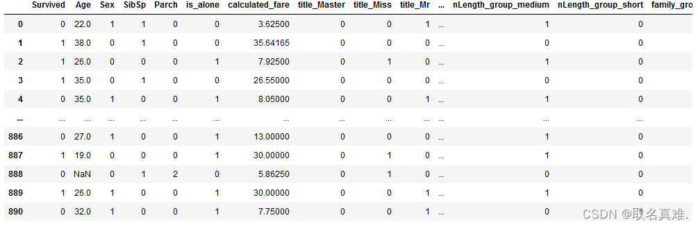
4.7用RandomForestRegressor预测年龄填补缺失数据
#用RandomForestRegressor预测年龄
# Importing RandomForestRegressor
from sklearn.ensemble import RandomForestRegressor

## writing a function that takes a dataframe with missing values and outputs it by filling the missing values.
def completing_age(df):
    ## gettting all the features except survived
    age_df = df.loc[:,"Age":]

    temp_train = age_df.loc[age_df.Age.notnull()] ## df with age values
    temp_test = age_df.loc[age_df.Age.isnull()] ## df without age values

    y = temp_train.Age.values ## setting target variables(age) in y
    x = temp_train.loc[:, "Sex":].values

    rfr = RandomForestRegressor(n_estimators=1500, n_jobs=-1)
    rfr.fit(x, y)

    predicted_age = rfr.predict(temp_test.loc[:, "Sex":])

    df.loc[df.Age.isnull(), "Age"] = predicted_age


    return df

## Implementing the completing_age function in both train and test dataset.
completing_age(train)
completing_age(test);

## Let's look at the his
plt.subplots(figsize = (22,10),)
sns.distplot(train.Age, bins = 100, kde = True, rug = False, norm_hist=False);
## create bins for age
def age_group_fun(age):
    """
    This function creates a bin for age
    """
    a = ''
    if age <= 1:
        a = 'infant'
    elif age <= 4:
        a = 'toddler'
    elif age <= 13:
        a = 'child'
    elif age <= 18:
        a = 'teenager'
    elif age <= 35:
        a = 'Young_Adult'
    elif age <= 45:
        a = 'adult'
    elif age <= 55:
        a = 'middle_aged'
    elif age <= 65:
        a = 'senior_citizen'
    else:
        a = 'old'
    return a

## Applying "age_group_fun" function to the "Age" column.
train['age_group'] = train['Age'].map(age_group_fun)
test['age_group'] = test['Age'].map(age_group_fun)

## Creating dummies for "age_group" feature.
train = pd.get_dummies(train,columns=['age_group'], drop_first=True)
test = pd.get_dummies(test,columns=['age_group'], drop_first=True);
五、建模
# separating our independent and dependent variable
X = train.drop(['Survived'], axis = 1)
y = train["Survived"]

from sklearn.model_selection import train_test_split
X_train, X_test, y_train, y_test = train_test_split(X, y,test_size = .33, random_state=0)

# Feature Scaling 数据差异大,进行标准化
## We will be using standardscaler to transform
from sklearn.preprocessing import StandardScaler
std_scale = StandardScaler()

## transforming "train_x"
X_train = std_scale.fit_transform(X_train)
## transforming "test_x"
X_test = std_scale.transform(X_test)

## transforming "The testset"
#test = st_scale.transform(test)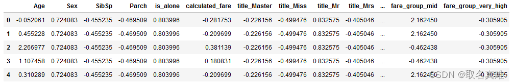
5.1LogisticRegression建模
##LogisticRegression建模

# import LogisticRegression model in python.
from sklearn.linear_model import LogisticRegression
from sklearn.metrics import mean_absolute_error, accuracy_score

## call on the model object
logreg = LogisticRegression(solver='liblinear',
                            penalty= 'l1',random_state = 42

                            )

## fit the model with "train_x" and "train_y"
logreg.fit(X_train,y_train)

y_pred = logreg.predict(X_test)

from sklearn.metrics import classification_report, confusion_matrix
# printing confision matrix
pd.DataFrame(confusion_matrix(y_test,y_pred),
            columns=["Predicted Not-Survived", "Predicted Survived"],
            index=["Not-Survived","Survived"] )

'''结果:
 	Predicted Not-Survived 	Predicted Survived
Not-Survived 	156 	           28
Survived 	     26 	           85
'''
from sklearn.metrics import classification_report, balanced_accuracy_score
print(classification_report(y_test, y_pred))
'''结果:
precision recall f1-score support
0 0.86 0.85 0.85 184
1 0.75 0.77 0.76 111
accuracy 0.82 295
macro avg 0.80 0.81 0.81 295
weighted avg 0.82 0.82 0.82 295
'''
from sklearn.metrics import accuracy_score
accuracy_score(y_test, y_pred)
#结果:0.81694915254237295.2Decision Tree建模
##Decision Tree建模
from sklearn.model_selection import RandomizedSearchCV
from sklearn.model_selection import GridSearchCV, StratifiedKFold, StratifiedShuffleSplit
from sklearn.model_selection import GridSearchCV
from sklearn.tree import DecisionTreeClassifier
max_depth = range(1,30)
max_feature = [21,22,23,24,25,26,28,29,30,'auto']
criterion=["entropy", "gini"]

param = {'max_depth':max_depth,
         'max_features':max_feature,
         'criterion': criterion}
grid = GridSearchCV(DecisionTreeClassifier(),
                                param_grid = param,
                                 verbose=False,
                                 cv=StratifiedShuffleSplit(n_splits=20, random_state=15),
                                n_jobs = -1)
grid.fit(X, y)


print( grid.best_params_)
print (grid.best_score_)
print (grid.best_estimator_)
'''结果:
{'criterion': 'entropy', 'max_depth': 5, 'max_features': 30}
0.828888888888889
DecisionTreeClassifier(criterion='entropy', max_depth=5, max_features=30)
'''

dectree_grid = grid.best_estimator_
## using the best found hyper paremeters to get the score. 最好的模型参数
dectree_grid.score(X,y)

#结果:0.8585858585858586
5.3randomforest建模
##randomforest建模
from sklearn.model_selection import GridSearchCV, StratifiedKFold, StratifiedShuffleSplit
from sklearn.ensemble import RandomForestClassifier
n_estimators = [140,145,150,155,160];
max_depth = range(1,10);
criterions = ['gini', 'entropy'];
cv = StratifiedShuffleSplit(n_splits=10, test_size=.30, random_state=15)


parameters = {'n_estimators':n_estimators,
              'max_depth':max_depth,
              'criterion': criterions

        }
grid = GridSearchCV(estimator=RandomForestClassifier(max_features='auto'),
                                 param_grid=parameters,
                                 cv=cv,
                                 n_jobs = -1)
grid.fit(X,y)

print (grid.best_score_)
print (grid.best_params_)
print (grid.best_estimator_)
'''结果:
0.8384328358208956
{'criterion': 'entropy', 'max_depth': 7, 'n_estimators': 160}
RandomForestClassifier(criterion='entropy', max_depth=7, max_features='auto',
                       n_estimators=160)
'''

rf_grid = grid.best_estimator_
rf_grid.score(X,y)
#结果:0.8742985409652076
5.4Adaboost建模
from sklearn.tree import DecisionTreeClassifier
from sklearn.ensemble import AdaBoostClassifier

# 创建一个决策树分类器作为基本估计器
base_estimator = DecisionTreeClassifier()

# 创建AdaBoost分类器并将决策树分类器作为基本估计器
ada_boost = AdaBoostClassifier(base_estimator=base_estimator)

# 使用AdaBoost分类器进行训练和预测
ada_boost.fit(X_train, y_train)

predictions = ada_boost.predict(X_test)

from sklearn.metrics import accuracy_score

accuracy_score(y_test, y_pred)
#结果:0.8169491525423729


from sklearn.model_selection import GridSearchCV
from sklearn.model_selection import StratifiedShuffleSplit

n_estimators = [80,100,140,145,150,160, 170,175,180,185];
cv = StratifiedShuffleSplit(n_splits=10, test_size=.30, random_state=15)
learning_r = [0.1,1,0.01,0.5]

parameters = {'n_estimators':n_estimators,
              'learning_rate':learning_r

        }

base_estimator = DecisionTreeClassifier()

grid = GridSearchCV(AdaBoostClassifier(base_estimator= base_estimator, ## If None, then the base estimator is a decision tree.
                                     ),
                                 param_grid=parameters,
                                 cv=cv,
                                 n_jobs = -1)
grid.fit(X,y)

ada_grid = grid.best_estimator_
ada_grid.score(X,y)
#结果:0.9887766554433222
原文地址:https://blog.csdn.net/qq_74156152/article/details/135424043
本文来自互联网用户投稿,该文观点仅代表作者本人,不代表本站立场。本站仅提供信息存储空间服务,不拥有所有权,不承担相关法律责任。
如若转载,请注明出处:http://www.7code.cn/show_55528.html
如若内容造成侵权/违法违规/事实不符,请联系代码007邮箱:suwngjj01@126.com进行投诉反馈,一经查实,立即删除!
主题授权提示:请在后台主题设置-主题授权-激活主题的正版授权,授权购买:RiTheme官网
声明:本站所有文章,如无特殊说明或标注,均为本站原创发布。任何个人或组织,在未征得本站同意时,禁止复制、盗用、采集、发布本站内容到任何网站、书籍等各类媒体平台。如若本站内容侵犯了原著者的合法权益,可联系我们进行处理。

![[PyTorch][chapter 5][李宏毅深度学习][Classification]](http://www.7code.cn/wp-content/themes/ripro-v2/assets/img/thumb-ing.gif)