manhattan:曼哈顿距离,又称城市街区距离,它的计算方式有点类似于只能90度拐角的街道长度。D
(
x
,
y
)
=
∑
i
=
1
k
∣
x
i
−
y
i
∣
D(x,y)=sum_i=1^k|x_i-y_i|
D(x,y)=i∑=1k∣xi−yi∣
chebyshev:chebyshev距离是两个数值向量在单个维度上绝对值差值最大的那个值。D
(
x
,
y
)
=
max
i
(
∣
x
i
−
y
i
∣
)
D(x,y)=text{max}_i(|x_i-y_i|)
D(x,y)=maxi(∣xi−yi∣)
metrics = ['minkowski', 'euclidean', 'manhattan', 'chebyshev' ]
acc_list = []

for metric in metrics:  # 遍历距离度量类型
    model = KNeighborsClassifier(metric = metric)
    model.fit(x_train, y_train)  # 记录训练数据
    p_test = model.predict(x_test)  # 预测测试图片
    accuracy = accuracy_score(p_test, y_test)  # 计算准确率
    acc_list.append(accuracy)
    print('metric: {}, accuracy: {:<.4f}'.format(metric, accuracy))
结果:
metric: minkowski, accuracy: 0.6969
metric: euclidean, accuracy: 0.6969
metric: manhattan, accuracy: 0.6920
metric: chebyshev, accuracy: 0.4090
绘制柱状图,可视化表示:
plt.bar(metrics, acc_list)  # 画图
plt.show()
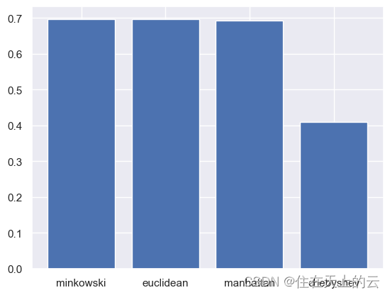
由上图可见,minkowski, euclidean, manhattan三种举例向量效果类似, chebyshev效果明显较差。
5.3 平均和加权KNN的区别
-
uniform: 平均KNN,这意味着所有的邻居节点在投票过程中具有相同的权重。也就是说,每个邻居节点对最终结果的影响是一样的,不考虑它们与查询点的距离。 -
distance:加权KNN,这意味着邻居节点的权重与它们到查询点的距离成反比。也就是说,距离查询点更近的邻居节点将对最终结果有更大的影响,而距离较远的邻居节点的影响较小。
weights = ['uniform', 'distance']
acc_list = []

for weight in weights:
    model = KNeighborsClassifier(weights = weight)
    model.fit(x_train, y_train)  # 记录训练数据
    p_test = model.predict(x_test)  # 预测测试图片
    accuracy = accuracy_score(p_test, y_test)  # 计算准确率
    acc_list.append(accuracy)
    print('metric: {}, accuracy: {:<.4f}'.format(metric, accuracy))
结果:
metric: chebyshev, accuracy: 0.6969
metric: chebyshev, accuracy: 0.7016
绘制柱状图,可视化表示:
plt.bar(weights, acc_list)  # 画图
plt.show()
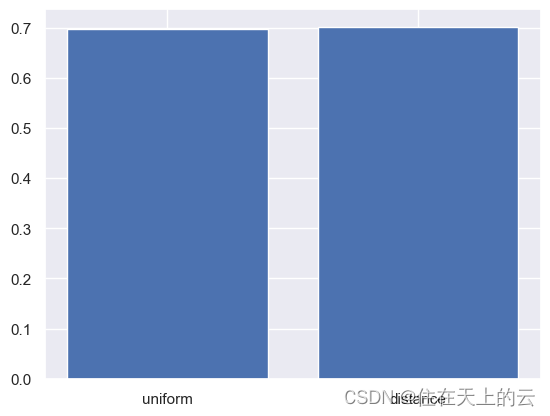
由上图可见,平均与加权结果类似,加权效果较好于平均KNN。
5.4 训练集大小对模型效果的影响
train_range = [1, 5, 10, 20, 50, 100, 200, 400, 600]
acc_lst = list()

for train_num in train_range:
    x_train, y_train = readFile(path_train, train_num)
    model = KNeighborsClassifier()
    model.fit(x_train, y_train)
    p_test = model.predict(x_test)
    accuracy = accuracy_score(p_test, y_test)
    acc_lst.append(accuracy)
    print('train: {}, accuracy: {:<.4f}'.format(train_num, accuracy))
结果:
train: 1, accuracy: 0.1972
train: 5, accuracy: 0.4264
train: 10, accuracy: 0.5035
train: 20, accuracy: 0.5906
train: 50, accuracy: 0.6568
train: 100, accuracy: 0.6707
train: 200, accuracy: 0.7005
train: 400, accuracy: 0.7065
train: 600, accuracy: 0.7025
绘制折线图,可视化表示:
plt.plot(train_range, acc_lst)
plt.xlabel('train')
plt.ylabel('Accuracy')
plt.show()
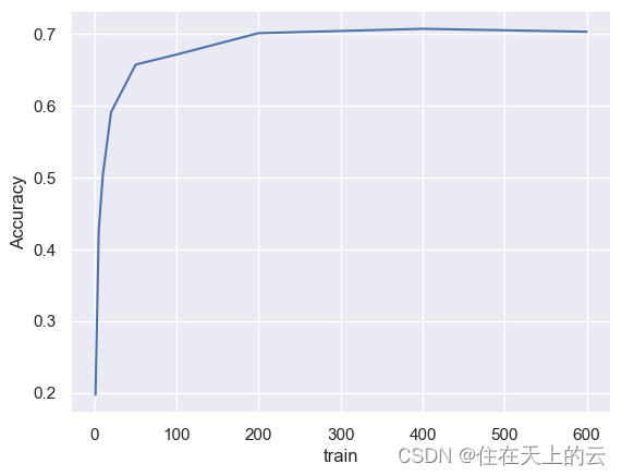
由上图可见,数据集数量越大,准确率越高,但是达到一定大小后增长变缓,甚至会有略微降低。
原文地址:https://blog.csdn.net/weixin_48024605/article/details/135974882
本文来自互联网用户投稿,该文观点仅代表作者本人,不代表本站立场。本站仅提供信息存储空间服务,不拥有所有权,不承担相关法律责任。
如若转载,请注明出处:http://www.7code.cn/show_64853.html
如若内容造成侵权/违法违规/事实不符,请联系代码007邮箱:suwngjj01@126.com进行投诉反馈,一经查实,立即删除!